Timely Dataflow and Total Order

06 Apr 2020

In anticipation of starting at Materialize, I’ve been reading through some of the fundamental literature that the product is built on. The first paper I’ve read through is Naiad: A Timely Dataflow System.

I enlisted the help of friends Forte Shinko and Ilia Chtcherbakov to help me work through it, and we ended up finding an interesting question that I’m not aware of a proof online for, so I’m going to share it today. There’s a decent amount of background we need to get through before we can even state the problem.

Timely Dataflow Graph Structure

Our first notion is of Timely Dataflow Graphs, defined in the paper as

Timely dataflow graphs are directed graphs with the constraint that the vertices are organized into possibly nested loop contexts, with three associated system-provided vertices. Edges entering a loop context must pass through an ingress vertex and edges leaving a loop context must pass through an egress vertex. Additionally, every cycle in the graph must be contained entirely within some loop context, and include at least one feed-back vertex that is not nested within any inner loop contexts.

Essentially, they look something like this, where the coloured boxes denote loop contexts:

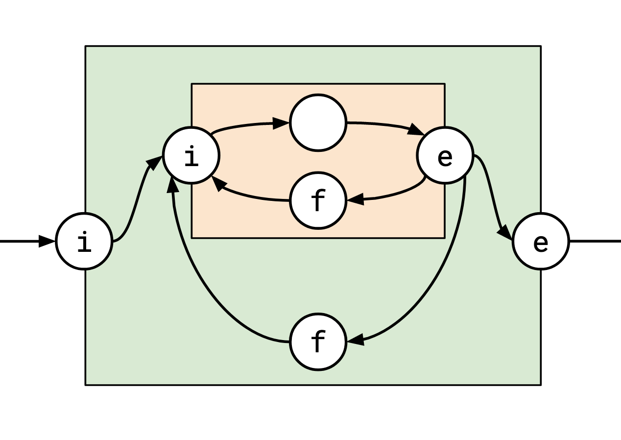
The important things to note are:

• the graph is directed,
• the vertices are organized into loop contexts,
• each vertex can be tagged either \(e\), \(i\), \(f\) (henceforth egress, ingress, and feedback), or have no tag at all,
• you must pass through an ingress vertex to enter a loop context, and an egress vertex to leave it.

We’ll revisit the bit about cycles later.

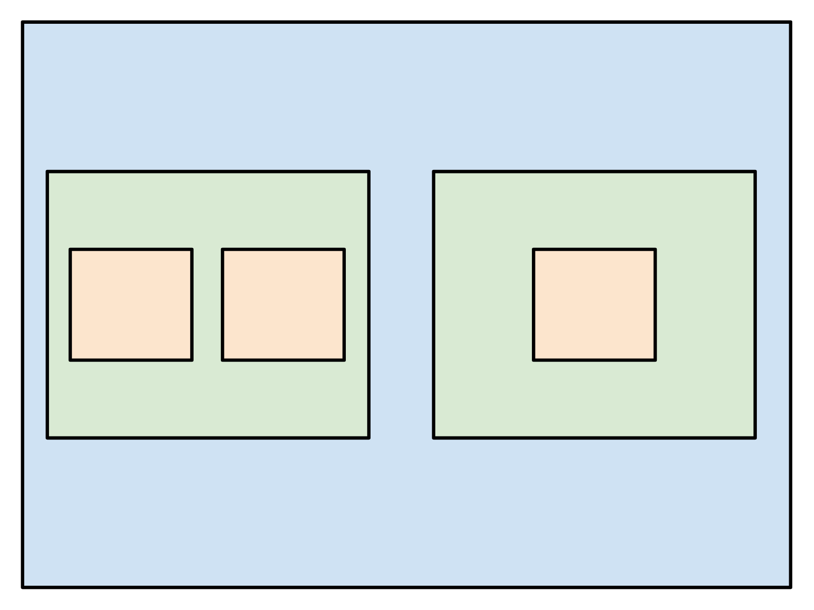
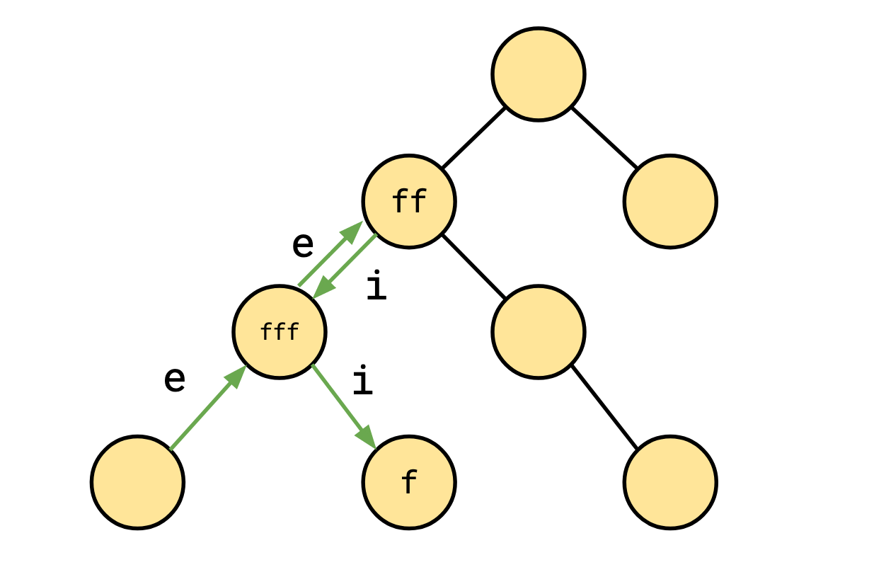
Since the loop contexts of a timely dataflow graph respect a hierarchy, they can be organized into a tree structure.

Consider this loop context structure (I’ve elided the vertices for simplicity):

This has this corresponding tree:

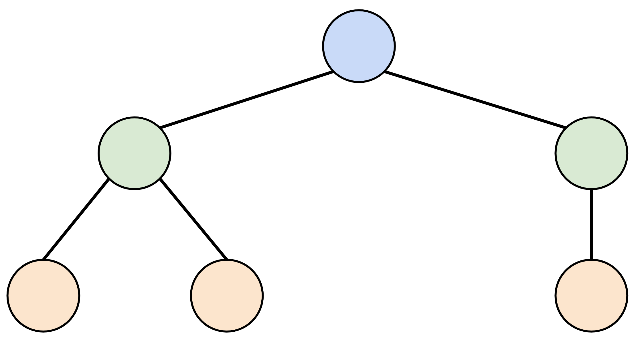
This is the dataflow graph’s loop context tree. We’ll see these a little later.

Timestamps and Paths

The structure of these graphs is all in service of messages passing through them. A message arrives in one end of a vertex and might (or might not) induce a message to be sent out the other end. These messages have timestamps. The timestamps are sequences of loop counters, each of which is a natural number: \[ \text{Timestamp} : \langle c_1, \ldots, c_k \rangle \in \mathbb N^k \]

Every vertex in the graph, when a message passes through it, modifies its timestamp in a specific way:

Vertex	Input Timestamp	Output Timestamp
Ingress	\(\langle c_1, \ldots, c_k \rangle\)	\(\langle c_1, \ldots, c_k, 0 \rangle\)
Egress	\(\langle c_1, \ldots, c_k, c_{k+1} \rangle\)	\(\langle c_1, \ldots, c_k \rangle\)
Feedback	\(\langle c_1, \ldots, c_k \rangle\)	\(\langle c_1, \ldots, c_k+1 \rangle\)

In English, ingress vertices add a new index, egress vertices remove the last index, and feedback vertices increment the last index. It might help you to recognize that the timestamps behave like a stack: ingress is a push operation, egress is a pop operation, and feedback peeks at the thing at the top and increments it.

As a message travels through the graph, its timestamp will be advanced as it passes through various vertices. We can summarize what happens to a timestamp traveling along that path with a path summary of the composition of all the vertices passed through.

We can represent these path summaries as strings of the operations we see. For instance, the path summary representing passing through an ingress followed by a feedback vertex will be denoted \(if\).

We’ll notate these operations such that they apply on the right:

\[ \langle c_1, \ldots, c_k \rangle i = \langle c_1, \ldots, c_k, 0 \rangle \] \[ \langle c_1, \ldots, c_k, c_{k+1} \rangle e = \langle c_1, \ldots, c_k \rangle \] \[ \langle c_1, \ldots, c_k \rangle f = \langle c_1, \ldots, c_k+1 \rangle \]

This notation is nice because it means that if we have a path from \(a\) to \(b\) with path summary \(X\) and a path from \(b\) to \(c\) with path summary \(Y\), then the path summary of following the first path followed by the second path, walking from \(a\) to \(c\) is simply \(XY\). For instance, if \(X = if\) and \(Y = ei\), \(XY = ifei\) (a careful reader might ask if we know that this operation is associative, to which I will point out this is just function composition).

You might know that when you have a thing like this where you can smash two objects together as strings to get a new object, you have a monoid, and indeed, these path summaries are a monoid. For this reason I’m going to use \(1\) to represent the empty string (the path summary for the path that doesn’t go anywhere). That is, \(x1 = 1x = x\) for all \(x\).

There are two useful identities we can infer from the definition of this monoid:

1. If we ingress, and add a point to our timestamp, and then egress and remove it, it’s equivalent to doing nothing at all: \[ ie = 1 \]

2. If we feedback to increment a point, and then egress and remove it, it’s equivalent to just egressing, since we can’t see the feedback anymore: \[ fe = e \]

These two identities actually define the monoid; our monoid is precisely: \[ \langle e,i,f: ie=1, fe=e \rangle. \]

These identities have an interesting property: in every scenario, they let us push all the \(e\)s in any string all the way to the left, getting a canonical form for any string, for example:

\[ ieeiffieeif = eif \]

So as a regular expression, every path can be canonically expressed in the form \[ e^* f^* (if^* )^*. \]

On to Order

Timestamps are totally ordered lexicographically (the natural “alphabetic” way). We can use this order to then define an order \(\le\) on path summaries: \[ p \le q \text{ if and only if } tp \le tq \text{ for all } t : \text{Timestamp} \] Put in words, a path summary \(p\) is \(\le\) a path summary \(q\) if \(p\) always advances a timestamp less than \(q\) does. This definition raises a question: for every distinct pair \(p\) and \(q\), is it the case that at least one of them is ordered before the other?

The answer is no. Here’s an example: \[ \begin{aligned} a &= 1 \cr b &= eeiffi \cr t_1 &= \langle 5, 5, 0 \rangle \cr t_2 &= \langle 5, 0, 0 \rangle \cr t_1a &= \langle 5, 5, 0 \rangle \cr t_2a &= \langle 5, 0, 0 \rangle \cr t_1b &= \langle 5, 2, 0 \rangle \cr t_2b &= \langle 5, 2, 0 \rangle \cr \end{aligned} \] And we have \(t_1a > t_1b\) but \(t_2a < t_2b\). So path summaries are only partially ordered. However! This brings us to the point at hand. The following sentence appears in the Timely paper:

The structure of timely dataflow graphs ensures that, for any locations \(l_1\) and \(l_2\) connected by two paths with different summaries, one of the path summaries always yields adjusted timestamps earlier than the other.

And this, dear reader, is the claim we are here to verify:

The set of path summaries for paths connecting two fixed vertices is totally ordered under \(\le\).

The Proof

As a note, I’m not going to be super formal here, I’m going to make some leaps that I think are justified in the interest of trying to make the argument here intuitive.

We have two vertices in a timely dataflow graph, \(u\) and \(v\) with two path summaries connecting them, \(X\) and \(Y\), and we want to show that at least one of these is true:

• \(X \le Y\)
• \(Y \le X\).

In fact, we will show a slightly stronger fact: let \(S_A\) and \(S_B\) be strings representing the normalized path summaries for two paths \(A\) and \(B\), connecting two fixed vertices. Then \(A \le B\) if and only if \(S_A \le S_B\) lexicographically (with \(e > f > i\)). This is quite a useful fact, because not only would it verify the truth of total-orderedness, but it gives us an algorithm for comparing two path summaries.

Before we continue, let’s get some intuition for what these normalized path summaries look like. Here are some examples of them (we use exponentials to notate repeated elements: \( e^n = \underbrace{e\cdots e}_{n \text{ times}} \), \(x^0 = 1\)): \[ \begin{aligned} &e^3fif^3if^2i \cr &e^2f^2if^3if^2i \cr &e^2f^0if^0if^3i \cr \end{aligned} \]

That we have a canonical form that looks like this is telling us something about how we should visualize path summaries.

Each \(e\) is us stepping out of a loop context, up a level in the loop context tree (since that’s how the dataflow graphs are structured), and each \(i\) is us stepping into a loop context. Every normalized path summary has a “rising” part of only \(e\)s, and a “falling” part of only \(i\)s and \(f\)s. In the “falling” part, each time we step down a level, we’ll hit some number of \(f\)s before stepping down again.

That means we should envision them as a rise and descent through the loop context tree. While a path originally might go up and down multiple times before eventually settling on where it’s going, the normalized form shows that this doesn’t really matter for our purposes. We could make this idea more precise but it’s a bit clunky, so I’m just going to stick with this vague notion of “every path basically looks like one of these cases.”

Consider the normalized path summary \[ e^2f^2if^3if^1. \]

This might correspond to a walk through a loop context tree that looks something like this:

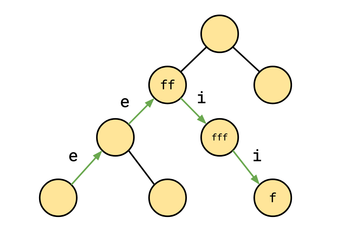
However, it could also look like this:

We’ll call the second kind, that revisits a loop context at some point a looping path.

It’s time to circle back to the structural property described in the Timely paper. They say:

Additionally, every cycle in the graph must be contained entirely within some loop context, and include at least one feedback vertex that is not nested within any inner loop contexts.

Let’s define the immediate loop context of a vertex or set of vertices as the smallest (lowest in the tree) loop context they’re contained in. Translating this from the paper into our terminology gives us the loop condition:

• every cycle passes through at least one feedback vertex whose immediate loop context is the same as the cycle’s immediate loop context.

However! This is not actually sufficient to prove the theorem. I think there are some additional structural constraints not stated explicitly in the paper. We’re going to change this slightly, to:

• every cycle or path from an egress vertex to an ingress vertex for the same loop context passes through at least one feedback vertex whose immediate loop context is the same as the cycle or path’s immediate loop context.

In other words, if we leave a loop context, then find our way back to that same loop context, we will hit a feedback vertex at the highest level that path hits. Since every looping path does this, every looping path hits a feedback vertex at its highest level. In terms of our normalized path summaries, the normalized path summary for any looping path always has an \(f\) immediately following the initial string of \(e\)s.

We’re now ready to break things down into cases. Remember, we’re trying to show that two paths \(A\) and \(B\) (having normalized path summaries \(S_A\) and \(S_B\)) are comparable.

Case 1: \(S_A\) and \(S_B\) have the same number of \(e\)s at the front

Since both \(A\) and \(B\) both end up in the same place, they both take the same path along the loop context tree (after getting rid of redundant side-tracks). This means that not only do they egress the same number of times, but they ingress the same number of times.

In fact they only differ in one way: the feedback vertices they hit on their journey down the loop context tree. So let the number of feedback vertices \(A\) hits at its top level \(a_1\), at the next level down \(a_2\), and so on, and the same for \(B\).

Then \[ \begin{aligned} S_A &= e^kf^{a_1}if^{a_2}\cdots if^{a_{r}} \cr S_B &= e^kf^{b_1}if^{b_2}\cdots if^{b_{r}} \cr \end{aligned} \]

If you work through what it looks like to apply one of these paths to a timestamp, you’ll see it looks like this: \[ \begin{aligned} \langle \ldots, n, c_1, \ldots c_k \rangle S_A &= \langle \ldots, n, c_1, \ldots c_k \rangle e^kf^{a_1}if^{a_2}\cdots if^{a_{r}} \cr &= \langle \ldots, n \rangle f^{a_1}if^{a_2}\cdots if^{a_{r}} \cr &= \langle \ldots, n + a_1, a_2, \ldots, a_{r} \rangle \cr \end{aligned} \]

And similarly,

\[ \langle \ldots, n, c_1, \ldots, c_k \rangle S_B = \langle \ldots, n + b_1, b_2, \ldots, b_{r} \rangle \]

so to compare these two all we have to do is compare the corresponding \(\langle a_1, \ldots, a_{r} \rangle \) tuples, which is what we said we had to do to compare the original strings lexicographically. So the lexicographic comparison here is sufficient, which is what we set out to show!

Case 2: One of \(S_A\) and \(S_B\) has more \(e\)s at front

Without loss of generality, assume \(S_A\) has more \(e\)s (egresses more) than \(S_B\). Since this means that \(S_A\) comes lexicographically after \(S_B\), we want to show that \(B \le A\).

Recall that paths have a rising part and a descending part in the loop context tree. Since \(A\) ultimately winds up in the same place as \(B\), it must rise, then double back (draw a picture of this scenario if you don’t believe me, it’s not too hard to convince yourself this is true). This means that \(A\) must be a looping path. So due to the loop condition, it hits a feedback vertex at the very apex of its journey. This means that we can guarantee that \(S_A\) looks like \(e^kfX\) for some \(X\) (rather than simply \(e^kX\)).

To better visualize this, applying \(S_A = e^kfX\) to a timestamp looks kind of like this:

\[ \begin{aligned} \langle \ldots , n, c_1, \ldots, c_k \rangle S_A &= \langle \ldots , n, c_1, \ldots, c_k \rangle e^k f X \cr &= \langle \ldots , n \rangle f X \cr &= \langle \ldots , n+1 \rangle X \cr &= \langle \ldots , n+1, d_1, \ldots \rangle \cr \end{aligned} \]

and applying \(S_B = e^rX\) looks kind of like this (\(r < k\)): \[ \begin{aligned} \langle \ldots , n, c_1, \ldots, c_k \rangle S_B &= \langle \ldots , n, c_1, \ldots, c_k \rangle e^r X \cr &= \langle \ldots , n, c_1, \ldots, c_{k-r} \rangle X \cr &= \langle \ldots , n, c_1, \ldots, c_{k-r}, \ldots \rangle \cr \end{aligned} \]

Since this comparison is lexicographic, the first place the two resulting timestamps differ is at the \(n\) vs. \(n + 1\) index, so that’s the comparison that will matter. Thus, \(S_A\) will always be greater, so \(B \le A\), as required.

All the symbols here make this look a little more complex than what’s actually going on: the idea is that given any timestamp, \(A\) reaches further back in it than \(B\) does, and then increments an index, so there’s no way \(B\) could make a timestamp bigger than \(A\) can.

And we’re done!

That concludes the proof; we have a total order for the path summaries connecting two vertices. It should be noted that this is not even a consideration in modern iterations of Timely Dataflow. What constitutes a “timestamp” and “path summary” is now sufficiently general that a total order is not needed or guaranteed, and there’s some interesting math to be done around that as well.

Thanks again to Forte and Ilia for their help investigating this problem, and thanks to the folks at Materialize for reading over this post for me!