Partially Ordered A*

19 Mar 2023

Tyler Glaiel recently posted a post on his Substack. I encourage you to read the whole post because it’s a great read, but I want to focus on the algorithmic problem he posted about. He shared his code that solves it, but I think it’s an interesting enough problem that it deserves some closer attention.

I want to present a general-purpose algorithm that solves his problem and many related problems in a very clean way.

The Setting and Existing Solutions

First, let’s summarize his problem: he has cats living on a grid that want to pathfind from their current position on the grid to some target position, subject to some maximum distance they can travel (in this example, 5 squares).

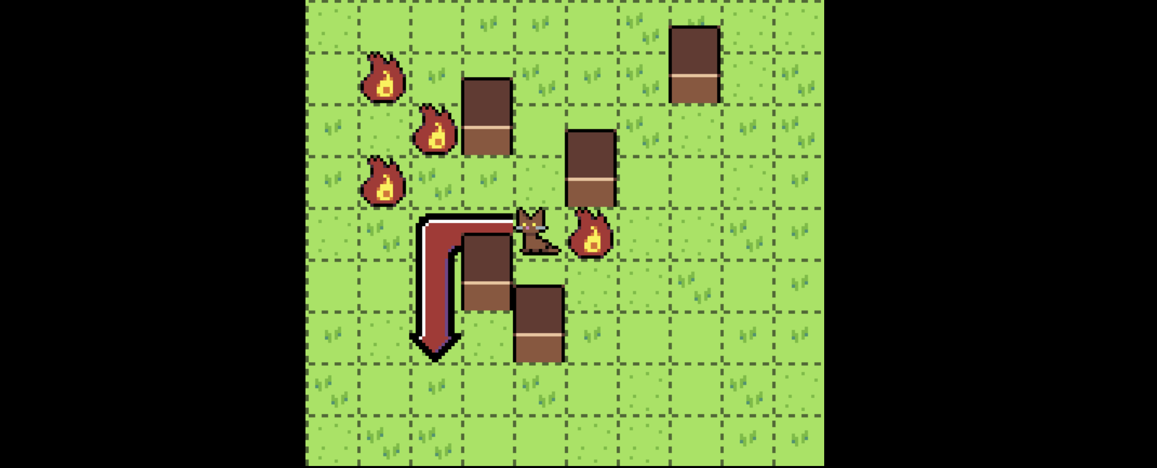
There are some squares that have fire on them. Cats can pass through fire, but they’d rather not. If a cat can reach the target square without passing through fire, they will pick a path that does so, even if it’s longer than the optimal path. If they must pass through fire to reach the target, they will.

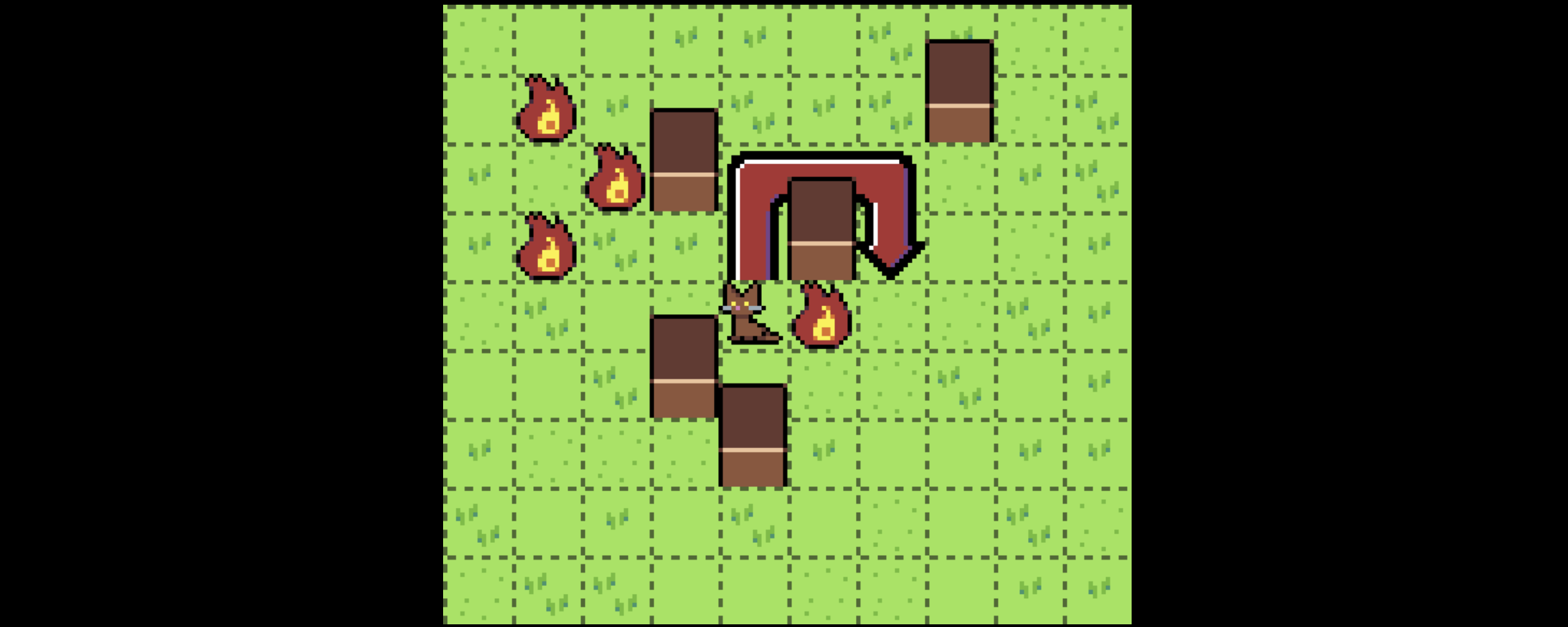
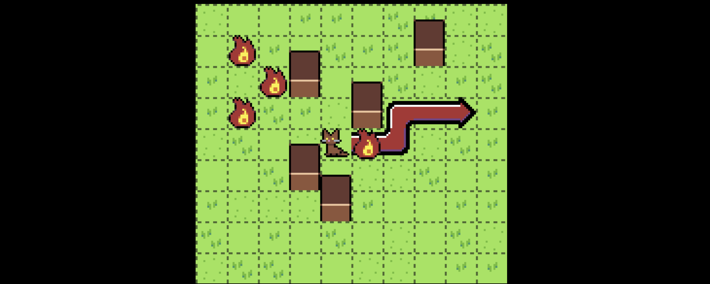
As Tyler says in his post, this problem looks very simple, but if you try to apply traditional pathfinding algorithms to it they will not work quite right. However, it turns out there is a generalization of those pathfinding algorithms that will solve this problem.

Classical A* pathfinding is a pretty natural variation on BFS or DFS, it’s just that the data structure used to store the frontier of vertices is not a queue or a stack, but a priority queue. That priority queue is ordered by the sum of:

• the distance travelled so far from the starting location, and
• a “heuristic,” which is some lower bound on how far we are from the goal (in this kind of grid-based pathfinding it’s common to use the Manhattan distance).

The first time we reach the goal node, we must have taken the shortest path, because any other potential path plus its lower bound must be larger than the path we just took (due to our use of a priority queue).

The Problem, and a Solution

Baked into this search algorithm is an assumption that gets violated by Tyler’s problem: if I reach a given location in two different ways, either those two ways have the same cost, or one is better for all purposes, meaning any path that goes through that square should take the same journey to get there, regardless of where it’s going afterwards.

You might recognize this as the Principle of Optimality: in any “big” problem, if you solve the “small” problems that make it up, the solutions to the small problems should themselves be optimal.

However, the setting of this problem invalidates this assumption. I think this subtle violation is the source of what makes this problem deceptively tricky. Consider the square marked with an X here:

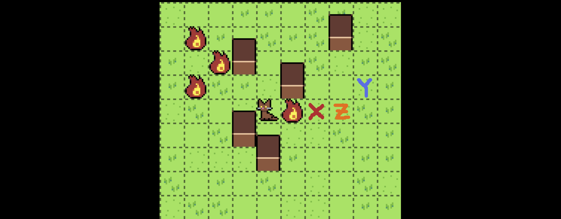
The best way to get to square X depends: if we’re trying to get to Z, we should go down and around the fire, since we can still get to Z with our movement range of 5.

If we’re trying to get to Y, however, we need to go through the fire, or else our movement range won’t allow us to reach it.

Thus, there are actually two “best” ways to get to X, neither of which can be considered strictly better than the other, and they have costs

• {distance: 2, fire: 1}, and
• {distance: 4, fire: 0}.

This kind of relationship is called a partial order. Some costs are incomparable, like these two, while other costs are comparable. For instance, for all purposes, {distance: 3, fire: 1} is worse than {distance: 2, fire: 1}. So we don’t actually have to keep around every path, only the ones that are “best in class” and not comparable with each other.

It turns out “a set of elements in a partial order which are all mutually incomparable” is a well-understood object, it is an antichain.

We can visualize a set of paths to a particular square as points on a 2D grid:

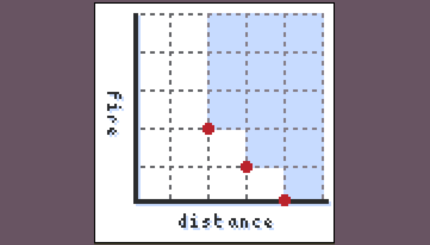
Any paths falling in the blue region (the upper set of the antichain) are irrelevant and strictly worse than this set of paths, while any paths outside of the blue region are an improvement on it.

There is a canonical way to turn a set of points into such an antichain, which is to just keep all the minimal points.

And it turns out this is approximately all the machinery we need to actually solve the problem:

• Do a search outwards from the starting location.
• Whenever you visit a new square and add the cost of traversal, you have to add it to each element of the cost antichain to construct a new one.
• Every time you visit a square, see what the antichain of costs we have for it is. If you can improve it, update it and add it to your frontier of points to explore.
• Once you’re done and no further updates are occurring, look at the antichain of possible costs on the goal square and pick out whichever one you like best (in this case, it would be the one with the lowest fire value).

For the setting described, with movement capped at five or six squares, this is probably fine. As Tyler mentions though, he wants to use A*, and it turns out we can extend A* to work in this setting as well.

Partially Ordered A*

As we said before, the point of A* is that we can usually use a heuristic to get a decent idea of which squares to visit first. If that heuristic has a particular nice property (namely that it’s always a lower bound on the distance), then it turns out we can ensure optimality while restricting our search space in this way.

The generalization to partially ordered costs works approximately the same way: we maintain a frontier of points to visit tagged with their current distance plus a lower bound, but now, since our costs aren’t totally ordered, we don’t have a canonical next point to visit:

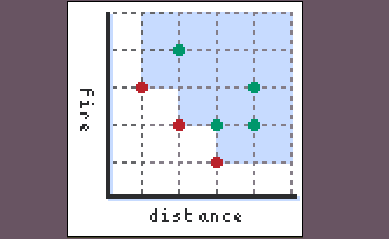
We instead can visit any points in the set’s lower antichain, that is, any of the red points in this diagram.

Now, when a path reaches the destination, it’s not “the best overall path” (since such a path might not exist), but it is better than any path in its upper set. So, unlike traditional A* where we simply terminate the algorithm when this happens, in this version, we delete all points from our frontier which are greater than the path that just concluded, and continue (notice that in the case where costs are totally ordered this is just the normal algorithm, where we terminate). We can safely delete these paths because our use of a lower bound ensures they have no way of ever “catching up” to the path that just concluded.

The cool thing about this algorithm (assuming you have data structures to store all these objects nicely) is that it works for any partially ordered set, which makes it really general and useful in a lot of scenarios.

I’ve skipped over a bunch of details here (in particular, various assumptions about how costs behave), for a more rigorous treatment of this idea of partially ordered costs for graph traversal, see my friend Ilia’s post on the topic.