Joins 13 Ways
03 Jul 2023Relational (inner) joins are really common in the world of databases, and one weird thing about them is that it seems like everyone has a different idea of what they are. In this post I’ve aggregated a bunch of different definitions, ways of thinking about them, and ways of implementing them that will hopefully be interesting. They’re not without redundancy, some of them are arguably the same, but I think they’re all interesting perspectives nonetheless.
Table of Contents
- A join is a lookup
- A join is a nested loop over rows
- A join is a nested loop over columns
- A join is compatible alternate realities
- A join is flatMap
- A join is the solution to the N+1 problem
- A join is paths through a graph
- A join is a minimal model
- A join is typechecking
- A join is an operation in the Set monad
- A join is the biggest acceptable relation
- A join is a…join
- A join is a ring product
A join is a lookup
The first and most practical way to see a join is that it’s “looking something up,” or adorning some data with some additional, redundant data.
I think the first place people typically encounter joins is when some guy on the internet has told them to normalize their tables. Meaning they’ve been told to stop storing data like this:
| user | country | country_code |
|---|---|---|
| Smudge | Canada | CA |
| Sissel | Canada | CA |
| Petee | United States | US |
This is “bad,” because there’s redundancy: country_code doesn’t change between rows with the same country. If we were storing something more volatile than this, we’d have to make sure that any changes to the data were reflected everywhere, which is error prone and inefficient.
The correct way to do this is to normalize the table. Create a table which only relates country and country_code:
| country_id | country | country_code |
|---|---|---|
| 1 | Canada | CA |
| 2 | United States | US |
and then reference that in the “fact table:”
| user | country_id |
|---|---|
| Smudge | 1 |
| Sissel | 1 |
| Petee | 2 |
Then a join is the operation that lets us recover the original table, which we might want to do some computations: to join these two tables we’d write:
SELECT user, country, country_code FROM
    users
      INNER JOIN
    countries
      ON users.country_id = countries.country_id
Going forward, we will often adopt that convention that we implicitly join “on” any columns of the two relations that have the same name. But we will play a bit fast and loose with this, don’t sweat the details too much.
A join is a nested loop over rows
Given some predicate p, the join of two sets R and S is:
def join(R, S, p):
  output = []
  for r in R:
    for s in S:
      if p(r, s):
        output.push((r, s))
  return output
If the cross product of two collections is all concatenations of rows from the two of them, their join is a subset of that.
A join is a nested loop over columns
The domain of a column is the set of possible values that can appear in it.
If I have a relation R whose columns are a and b, and S whose columns are b and c, then the join of R and S is:
def join(R, S):
  output = []
  for a in domain(a):
    for b in domain(b):
      for c in domain(c):
        if R.contains(a, b) and S.contains(b, c):
          output.push([a, b, c])
  return output
A join is compatible alternate realities
Here’s our first weird one.
John and Sally are standing around the corner from each other, each has a pet, and each can see a stray animal on the corner, but they can’t see each other.
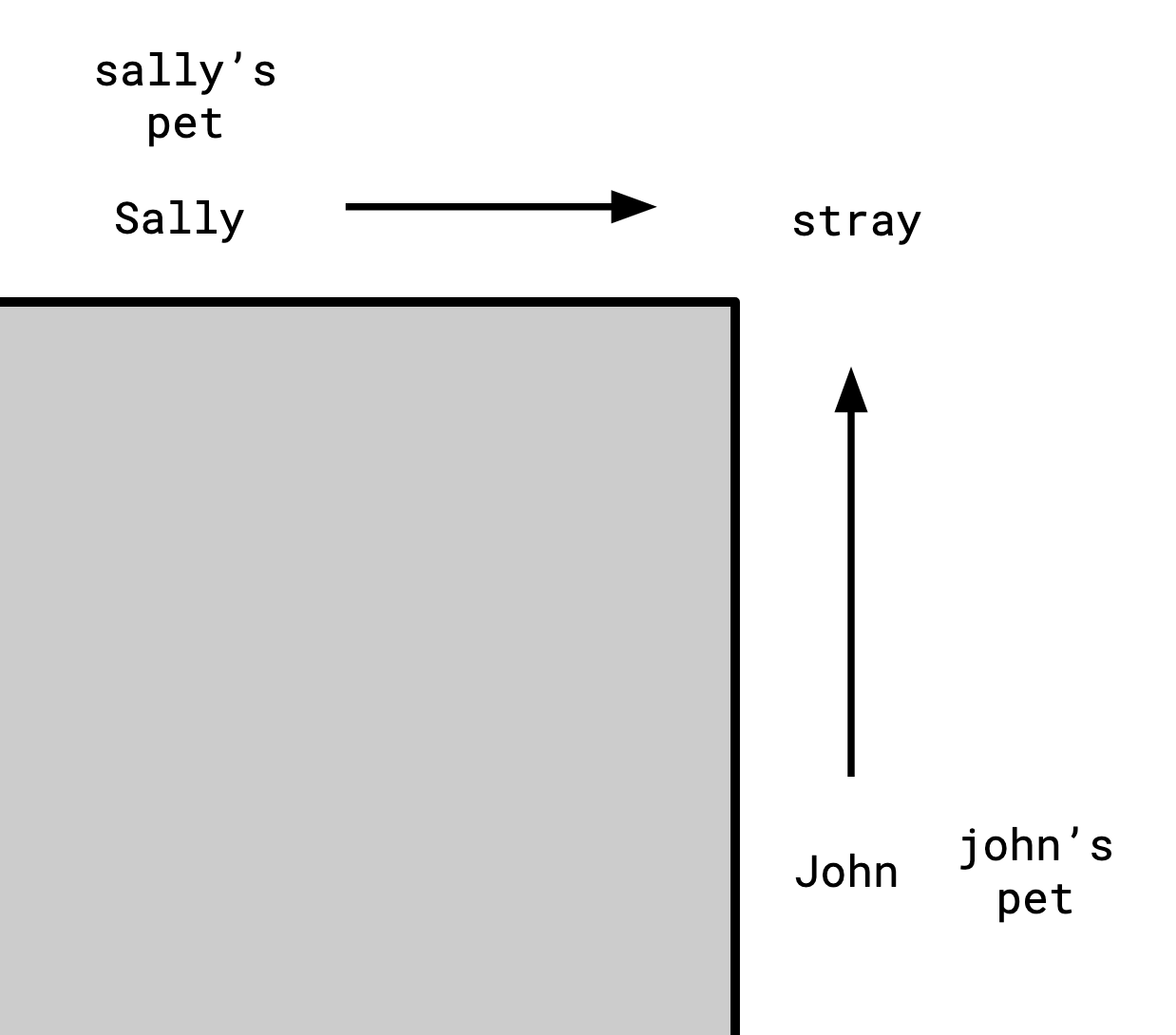
John and Sally both exist in a handful of alternate realities at once. For instance, there’s one reality where John has a dog, and another where he has a cat. We can summarize the realities that are possible for John in a relation:
| john’s pet | stray |
|---|---|
| dog | dog |
| cat | dog |
| cat | mouse |
Similarly, Sally also has a pet, and can also see the stray:
| sally’s pet | stray |
|---|---|
| dog | mouse |
| cat | mouse |
| mouse | dog |
We only have this imperfect information, because John can’t see Sally’s pet, and Sally can’t see John’s pet.
We can still make some inferences though: it can’t be the case that John has a dog while Sally has a cat, because then they would disagree on what the stray was (whenever John has a dog, the stray is a dog, but whenever Sally has a cat, the stray is a mouse).
By this logic, we can list out all the combinations that might exist:
| john’s pet | stray | sally’s pet |
|---|---|---|
| dog | dog | mouse |
| cat | dog | mouse |
| cat | mouse | dog |
| cat | mouse | cat |
This is the join of the two tables on stray.
A join is flatMap
The flatMap function in many programming languages operates on arrays.
It computes a new array for every element of the original, and concatenates the results.
> [1, 2, 3].flatMap(x => new Array(x).fill(x))
[ 1, 2, 2, 3, 3, 3 ]
This can implement a join. This:
SELECT * FROM r INNER JOIN s ON p
becomes this:
r.flatMap(x => s.filter(y => p(x, y)))
Some SQL variants support a LATERAL construction which turns joins into flatMaps:
pg=# SELECT * FROM
  (VALUES (1), (2), (3)) r(x),
  LATERAL (SELECT * FROM generate_series(1, x)) u;
 x | generate_series
---+-----------------
 1 |               1
 2 |               1
 2 |               2
 3 |               1
 3 |               2
 3 |               3
(6 rows)
Whenever the right-hand side of such a flatMap doesn’t contain any references to the left-hand side, it’s equivalent to a cross product (this is the crux of how query decorrelation is done, utilizing successive rewrites to remove column references from the right-hand side).
A join is the solution to the N+1 problem
A common problem that occurs when using ORMs is called the “N+1 problem.” This happens when you need to do a query for each row in a result set. It ends up looking something like this:
pets = run_query("SELECT * FROM users")
for pet in pets:
  country_code = run_query(
    "SELECT country_code FROM countries WHERE country_id = %d" % pet.country_id
  )
  print(pet.name, country_code)
This is a really common problem that shows up when people aren’t yet used to using relational databases. The problem is that in databases that use connections, like Postgres (this is not so much of a problem for in-process databases like Sqlite), there’s a high fixed cost to an individual query. Thus, you might want a way to tell the database “please do all these lookups for me,” and the result turns out to be exactly a join:
SELECT name, country_code FROM
  users INNER JOIN countries ON users.country_id = countries.id
A join is paths through a graph
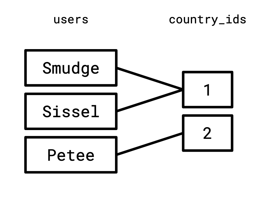
A relation is so named because it “relates” two sets.
In the case of our users table,
it relates the set of usernames with the set of country IDs.
We can visualize this relationship as a graph:
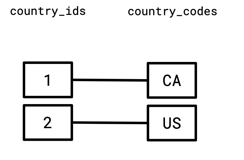
And similarly, we relate the set of country IDs to the set of two-letter country codes:
Since the right-hand side of the first graph, and the left-hand side of the second graph share a vertex set, it makes sense to consider them together:
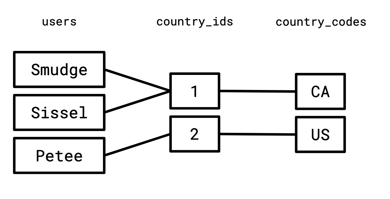
If we enumerate all the paths that start in the left set of this graph, go to a vertex in the middle set, and end on a vertex in the right set, we will construct exactly the join of these two relations.
A join is a minimal model
In formal logic, a model of a set of sentences is a set of facts which make all of the sentences true. In this setting, a relation is a predicate. The users relation is the predicate that satisfies the following:
users("Smudge", 1).
users("Sissel", 1).
users("Petee", 2).
and the country relation is the predicate that satisfies:
country(1, "Canada", "CA").
country(2, "United States", "US").
Now consider the following implication:
\[ \texttt{users}(a, b) \wedge \texttt{countries}(b, c, d) \rightarrow \texttt{Q}(a, b, c, d) \]
read “whenever users(A, B) and countries(B, C, D), then Q(A, B, C, D)." A model of this sentence is a set of facts which Q is true for such that this sentence is true.
One possible model is:
Q("Smudge", 1, "Canada", "CA").
Q("Smudge", 2, "United States", "US").
Q("Sissel", 1, "Canada", "CA").
Q("Sissel", 2, "United States", "US").
Q("Petee", 1, "Canada", "CA").
Q("Petee", 2, "United States", "US").
Another is
Q("Smudge", 1, "Canada", "CA").
Q("Smudge", 2, "United States", "US").
Q("Sissel", 1, "Canada", "CA").
Q("Sissel", 2, "United States", "US").
Q("Petee", 2, "Canada", "CA").
Q("Petee", 1, "United States", "US").
Q("Banana", 1, "Banana", "Banana").
It’s not particularly satisfying that this definition means we can have multiple possible models. We want something canonical. That’s why we ask for the smallest model that works. It turns out that for sentences like this, such a model always exists, and it’s the intersection of all models.
Here it’s
Q("Smudge", 1, "Canada", "CA").
Q("Sissel", 1, "Canada", "CA").
Q("Petee", 2, "United States", "US").
which is the join of users and country.
A join is typechecking
ML-style type systems bear a lot of similarities to joins (mostly because they very strongly resemble Prolog and Datalog). First, let’s define our relations as Rust traits:
trait Users {}
trait CountryCode {}
Now define our values, they’re Rust concrete types:
struct Smudge;
struct Sissel;
struct Petee;

struct Canada;
struct UnitedStates;

struct CA;
struct US;
impl Users for (Smudge, Canada) {}
impl Users for (Sissel, Canada) {}
impl Users for (Petee, UnitedStates) {}

impl CountryCode for (Canada, CA) {}
impl CountryCode for (UnitedStates, US) {}
Now we define the join itself.
A triple (A, B, C) is in the join when (A, B) is in Users, and (B, C) is in CountryCode.
trait UserCountryCode {}

impl<A, B, C> UserCountryCode for (A, B, C)
where
    (A, B): Users,
    (B, C): CountryCode,
{
}
Finally, we can check if something is in the join if our program typechecks. This typechecks:
fn test<X: UserCountryCode>() {}

fn main() {
    test::<(Smudge, _, CA)>()
}
While this doesn’t:
fn test<X: UserCountryCode>() {}

fn main() {
    test::<(Smudge, _, US)>()
}
error[E0277]: the trait bound `(Canada, US): CountryCode` is not satisfied
  --> src/main.rs:32:12
   |
32 |     test::<(Smudge, _, US)>()
   |            ^^^^^^^^^^^^^^^ the trait `CountryCode` is not implemented for `(Canada, US)`
   |
   = help: the following other types implement trait `CountryCode`:
             (Canada, CA)
             (UnitedStates, US)
note: required for `(Smudge, Canada, US)` to implement `UserCountryCode`
  --> src/main.rs:22:15
   |
22 | impl<A, B, C> UserCountryCode for (A, B, C)
   |               ^^^^^^^^^^^^^^^     ^^^^^^^^^
...
25 |     (B, C): CountryCode,
   |             ----------- unsatisfied trait bound introduced here
note: required by a bound in `test`
  --> src/main.rs:29:12
   |
29 | fn test<X: UserCountryCode>() {}
   |            ^^^^^^^^^^^^^^^ required by this bound in `test`
A join is an operation in the Set monad
Let’s define an option type (in JavaScript).
let Some = x => ({
    map: f => Some(f(x)),
    // Sometimes called `bind`.
    andThen: f => f(x),
    inspect: () => `Some(${JSON.stringify(x)})`,
});

let None = () => ({
    map: () => None(),
    andThen: () => None(),
    inspect: () => `None()`,
});
Now, say we have some records, but they’re all optional. As in, we might not
have them, so we have to wrap them in Some:
let user = Some({ name: 'Smudge', country: 'Canada' });
let country1 = Some({ country: 'Canada', code: 'CA' });
let country2 = Some({ country: 'United States', code: 'US' });
Now we’ll write a function that takes two of these records and returns Some of their merging if they’re compatible, and None otherwise:
let merge = (user, country) => {
    if (user.country === country.country) {
        return Some({ name: user.name, country: user.country, code: country.code });
    } else {
        return None();
    }
}
But since our actual records are optional, we need to wrap them in calls to andThen:
let combine = (user, country) => {
    return user.andThen(user => {
        return country.andThen(country => {
            return merge(user, country);
        })
    });
}
Now we can see the results of calling this function with various values:
console.log(combine(user, country1).inspect());
console.log(combine(user, country2).inspect());
console.log(combine(None(), country1).inspect());
console.log(combine(user, None()).inspect());
One interesting thing about the way we’ve set this up is that we can implement our “container” type differently, but keep the implementation.
Let’s implement a different container, called Rel, which stores a set of records.
Now our map operates on every row, and our andThen returns another relation,
which all get concatenated to the new relation.
let Rel = x => ({
    map: f => Rel(x.map(f)),
    andThen: f => Rel(x.flatMap(v => f(v).list())),
    list: () => x,
})
Now we can instantiate some data:
let users = Rel([
    { name: 'Smudge', country: 'Canada' },
    { name: 'Sissel', country: 'Canada' },
    { name: 'Petee', country: 'United States' },
]);

let countries = Rel([
    { country: 'Canada', code: 'CA' },
    { country: 'United States', code: 'US' },
]);
And try running the same function combine from before:
console.log(combine(users, countries).list());
And we get the join of the two relations:
[
  { name: 'Smudge', country: 'Canada', code: 'CA' },
  { name: 'Sissel', country: 'Canada', code: 'CA' },
  { name: 'Petee', country: 'United States', code: 'US' }
]
A join is the biggest acceptable relation
For two relations \(R\) and \(S\), say a third relation \(T\) which has all the columns from both is “acceptable” if it doesn’t invent any new information.
By that I mean, if you look at any row in \(T\) and restrict it to just the columns in \(R\), the resulting row exists in \(R\), and the same is true for \(S\).
For instance, say our tables are:
\(R\)
| user | country |
|---|---|
| Smudge | Canada |
| Sissel | Canada |
| Petee | United States |
\(S\)
| country | country_code |
|---|---|
| Canada | CA |
| United States | US |
This \(T\) is unacceptable:
| user | country | country_code |
|---|---|---|
| Smudge | Canada | US |
Because if we restrict to the columns of \(S\), \(\langle \texttt{country}, \texttt{country\_code} \rangle \), we get
| country | country_code |
|---|---|
| Canada | US |
Which doesn’t exist in \(S\).
Notably, the empty relation is acceptable. The largest acceptable relation, here, is
| user | country | country_code |
|---|---|---|
| Smudge | Canada | CA |
| Sissel | Canada | CA |
| Petee | United States | US |
This is the join of the two relations.
A join is a…join
A partial order is a set equipped with a binary relation \(\le\) satisfying the following properties:
- Reflexivity: \(a \le a\) for all \(a\),
- Antisymmetry: If \(a \le b\) and \(b \le a\), then \(a = b\), and
- Transitivity: If \(a \le b\) and \(b \le c\), then \(a \le c\).
(I provide this definition to be complete, but if it’s new to you, don’t expect the above to give you the intuition you’d need to actually be able to think about it.)
In a partial order, if two elements \(a, b\) always have a least upper bound (that is, a smallest \(x\) which \(a\) and \(b\) are both \(\le\)), then that is called their join and is written \(a \vee b\).
Define the following partial order on relations: \(R \le Q\) if:
- \(Q\) contains all the columns in \(R\), and
- restricting any row in \(Q\) to just the columns in \(R\) gives a row in \(R\).
Then for two relations \(R\) and \(S\), \(R \vee S\) exists, and it’s their join (in both senses of the word).
A join is a ring product
You might know from high school how to manipulate polynomials. If \(a\), \(b\), and \(c\) are all unknowns, the following expressions are all equivalent:
\[ a(b + c) = ab + ac = ba +ca = ca + ba = (c + b)a \]
We can represent a relation algebraically in this way. A row is the product of its columns. We represent the row
| user | country_id |
|---|---|
| Smudge | 1 |
as the product of two (column name, column value) pairs:
\[ [\text{user}=\texttt{Smudge}] [\text{country\_id}=\texttt{1}] \]
A relation is the sum of its rows:
\[ R = \begin{aligned} &[\text{user}=\texttt{Smudge}][\text{country\_id}=\texttt{1}] \cr +&[\text{user}=\texttt{Sissel}][\text{country\_id}=\texttt{1}] \cr +&[\text{user}=\texttt{Petee}][\text{country\_id}=\texttt{2}] \cr \end{aligned} \]
We also have the special value 1, satisfying \(1x = x\) for all \(x\).
We then add the following rules for simplifying these expressions:
Idempotence:
$$ [x = y][x = y] = [x = y] $$
and Contradiction:
$$ [x = y][x = z] = 0 \text{ if }y \not= z. $$
our lookup table here is
\[ S = \begin{aligned} &[\text{country\_id}=\texttt{1}][\text{country}=\texttt{Canada}][\text{country\_code}=\texttt{CA}] \cr +&[\text{country\_id}=\texttt{2}][\text{country}=\texttt{United States}][\text{country\_code}=\texttt{US}] \cr \end{aligned} \]
Then something interesting happens if we take the product of these two expressions, obeying the normal rules of polynomial rewriting such as distributivity:
\[ \begin{aligned} &RS = \cr &\left(\begin{aligned} &[\text{user}=\texttt{Smudge}][\text{country\_id}=\texttt{1}] \cr +&[\text{user}=\texttt{Sissel}][\text{country\_id}=\texttt{1}]\cr +&[\text{user}=\texttt{Petee}][\text{country\_id}=\texttt{2}] \cr \end{aligned}\right) \cr &\left( \begin{aligned} &[\text{country\_id}=\texttt{1}][\text{country}=\texttt{Canada}][\text{country\_code}=\texttt{CA}] \cr +&[\text{country\_id}=\texttt{2}][\text{country}=\texttt{United States}][\text{country\_code}=\texttt{US}] \cr \end{aligned} \right) \end{aligned} \]
If you apply the laws of distributivity and commutativity here, you’ll wind up with the following:
\[ \begin{aligned} &[\text{user}=\texttt{Smudge}][\text{country\_id}=\texttt{1}] [\text{country}=\texttt{Canada}] [\text{country\_code}=\texttt{CA}] \cr +&[\text{user}=\texttt{Sissel}][\text{country\_id}=\texttt{1}][\text{country}=\texttt{Canada}] [\text{country\_code}=\texttt{CA}]\cr +&[\text{user}=\texttt{Petee}][\text{country\_id}=\texttt{2}][\text{country}=\texttt{United States}] [\text{country\_code}=\texttt{US}] \cr \end{aligned} \]
Which is precisely the join of the two relations (I’m told this is a tensor contraction).