Compaction

You hear the word “log” a lot when talking about databases. This is because databases are fundamentally comprised of sin.

(Shared mutable state.)

Logs are natural in a setting where you want to be principled about your treatment of mutation because one way to think about mutation is how a variable starts from an initial value and undergoes several “transformations.”

This sequence of operations:

let x = 1;
x = x + 3;
let y = 7;
x = x * 2;

can be written to a log as a history of what operations were performed:

let ops = [
  ["set", "x", 1],
  ["plus", "x", 3],
  ["set", "y", 7],
  ["times", "x", 2],
];

we can then recover the final value of the database via a fold over the sequence of operations:

let apply = (value, op) => {
  switch (op[0]) {
    case "set":
      return {
        ...value,
        [op[1]]: op[2],
      };
    case "plus":
      return {
        ...value,
        [op[1]]: value[op[1]] + op[2],
      };
    case "times":
      return {
        ...value,
        [op[1]]: value[op[1]] * op[2],
      };
  }
};

console.log(ops.reduce(apply, {})); // => { x: 8, y: 7 }

And in fact, not just the final value, but we are able to recover any intermediate value we please by only applying a prefix of operations:

console.log(ops.slice(0, 2).reduce(apply, {})); // => { x: 4 }

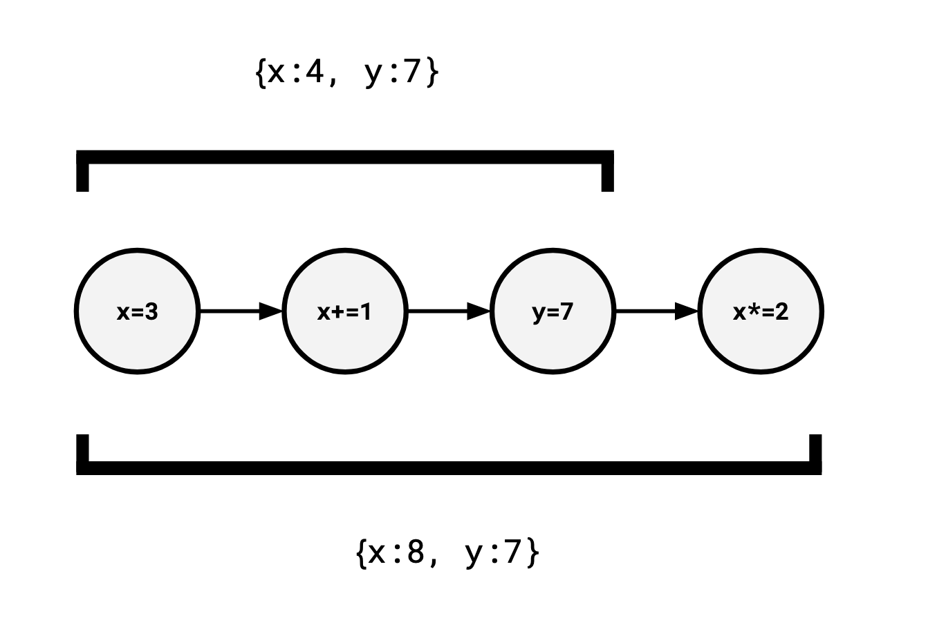
If we associate each operation with a timestamp, we can easily provide readers the ability to time travel by restricting them to whatever prefix they like:

let ops = [
  { t: 10, op: ["set", "x", 1] },
  { t: 20, op: ["plus", "x", 3] },
  { t: 30, op: ["set", "y", 7] },
  { t: 40, op: ["times", "x", 2] },
];

let read = (ops, at) => {
  let view = {};
  for (let { t, op } of ops) {
    if (t > at) {
      break;
    }
    view = apply(view, op);
  }
  return view;
};

console.log(read(ops, 25)); // => {x: 4}
console.log(read(ops, 31)); // => {x: 4, y: 7}

This is very useful if, for instance, we want to provide some particular consistency semantics (“users should not observe writes of users who showed up after them”) while still allowing concurrent writes (if new writes are assigned later timestamps, they are invisible to existing readers). This is the basic idea behind multiversion concurrency control, and is also the basis of how databases allow time travel queries.

I think of this as each event living along a big long timeline, and when a reader calls read(ops, n), they situate themselves at a position on the timeline and look backwards.

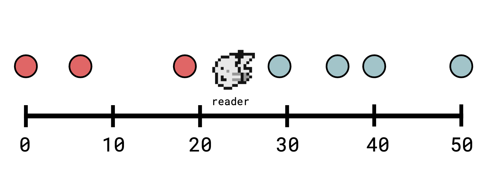
From the perspective of our observer, who is located at timestamp 23, the visible operations are those marked in red. Note that we use the convention that observers on a point x can see an entry also on x.

By keeping this log around for all eternity, we can permit readers to see what the state of the world was at whatever point in time they please. Of course, we might not want to do that. If our log looks something like this:

let ops = [
    {t: 10, ["set", "x", 1]},
    {t: 20, ["set", "x", 2]},
    {t: 30, ["set", "x", 3]},
    {t: 40, ["set", "x", 4]},
    {t: 50, ["set", "x", 5]},
    {t: 60, ["set", "x", 6]},
    {t: 70, ["set", "x", 7]},
    ...
];

and our users don’t care about what happened before a certain point in time, we can safely simplify our log to use less storage. If, say, users do not care (or are not permitted) to hop on the timeline at a timestamp earlier than 54, we can collapse everything from before then up to that point:

let ops = [
    {t: 54, ["set", "x", 5]},
    {t: 60, ["set", "x", 6]},
    {t: 70, ["set", "x", 7]},
    ...
];

and nobody can tell that we did so.

Breaking this down, we have:

• a set of events, each occurring at a point in time (a log), and
• a set of times we say we care about being able to time-travel to, say 54 and after (a vantage point) and
• we are transforming the log to something more space-efficient, which, given the vantage point, is logically equivalent.

By logically equivalent, I mean as long as a reader is adhering to the limitations we’ve enforced (“I will not read at times prior to 54"), they can’t tell the difference between the two representations.

This process of combining a log and a vantage point with this goal is called compaction. What we’ve done here is the simplest possible case for compaction: a single, advancing point over time. This is sometimes known as logical compaction, to contrast it with physical compaction, which is typically just reorganizing data, as you might when you defragment your hard drive.

Systems can utilize compaction in varying ways, in this post I’m going to outline two systems I’m familiar with to contrast their use of compaction.

Pebble

Pebble is an LSM created and used by CockroachDB, based off of RocksDB (and, by extension, LevelDB). Knowing how an LSM works is not essential to understand its use of compaction, effectively it works by appending writes to a log.

Every write is assigned a strictly increasing sequence number (for our purposes, this is a timestamp), and every read is performed by instantiating an iterator assigned a particular sequence number, which can see all the writes that occurred at timestamp \(\le\) its assigned timestamp (iterators are capable of seeks, which is how point reads are performed). This means that an iterator has a consistent view over the state of the database.

Pebble iterators don’t actually really interact with compaction: the immutable files they get their data from are all reference counted and will be kept around until the iterator is disposed of. This is typically not a problem since iterators are expected to be short-lived.

What if we need to be able to read from the same sequence number over a long period of time? This is an important use case for CockroachDB’s backup functionality, where they want to be able to read the state of the entire (potentially large) database. It’s not a good idea to keep an iterator open for an extremely long time, since, as noted, that prevents copies of data from being garbage collected.

To solve this, Pebble supports what it calls a snapshot. A snapshot of a sequence number x is “the ability to mint an iterator at sequence number x.” This is different from an iterator itself since we are not holding onto physical pieces of data, just informing Pebble that we want to read it at some point in the future (that is, we are logically holding onto the data). A user can request to create a snapshot, which Pebble will make note of and hand out a token for.

Unlike iterators, it’s reasonable to keep snapshots open for a long time, and also unlike iterators, they interact with Pebble’s ability to do compaction.

Snapshots (and iterators created absent a snapshot) have an important property: you can only create one at the most recent sequence number. You can never create a new snapshot at some point in the past. This means that in the absence of any outstanding snapshots, the vantage point of Pebble is always the newest sequence number \(t\): it’s impossible for anyone to read prior to it (ignoring iterators created in the past, which again, achieve this independently of compaction). What if we have snapshots open at sequence numbers \(S\) in the past? We now need to support reading at each of \(S \cup {t}\).

We could achieve this by doing the same thing we outlined in the intro: keep tracking the smallest sequence number in \(S\) and do not throw away any data occurring after that, but actually, we can do better here.

Remember our view of the log as a big long timeline where observers can stand. Say we have observers at \(S = \{s_1, s_2, s_3\} = \{13, 22, 45\}\):

We could simply compact everything from before t = 13 up to 13, leaving everything after 13 at full granularity, but we can do better: we can compact everything in between each pair. Compact everything in \((-\infty, 13]\) to 13, \((13, 22]\) to 22, \((22, 45]\) to 45, and everything else to the current open sequence number (say, 65).

Pebble calls these regions that can be collapsed to a point compaction stripes. The key observation here is that no observer can distinguish two points in the same stripe, so it’s always safe to compress them into a single point (“safe” meaning “no reader can tell that you did it”).

We say two timestamps \(a\) and \(b\) are indistinguishable if there’s no observer that can observe one but not the other. The timestamps within a given stripe are indistinguishable.

Another important observation is that “indistinguishability” is an equivalence relation, and one way to express such a relation is by a selector: a function \(\text{rep}\) such that:

• \(\text{rep}(x)\) and \(x\) are indistinguishable and
• \(\text{rep}(x) = \text{rep}(y)\) if and only if \(x\) and \(y\) are indistinguishable.

\(\text{rep}(x)\) is called the representative element for \(x\)’s equivalence class (the term “selector” comes from the fact that this function is “selecting” a distinguished element from each equivalence class).

In our case (having the current max sequence number as \(65\)), this selector is: $$ \text{rep}_{\{13,22,45\} \cup \{65\}}(t) = \begin{cases} 13 &\text{if } t \in (-\infty, 13] \cr 22 &\text{if } t \in (13, 22] \cr 45 &\text{if } t \in (22, 45] \cr 65 &\text{otherwise}\cr \end{cases} $$

So as before, we have

• a set of events (writes),
• a set of vantage points (the open snapshots), and
• we are transforming our log to something more space-efficient but equivalent, by fast-forwarding all points within a stripe to the same point (allowing redundant operations to be elided).

Differential Dataflow

Differential Dataflow (Differential) is a framework for incremental computation. The idea being that you can write a transformation over some input data, and as that input data changes, the output will be incrementally maintained.

One thing distinguishing Differential from many other systems is its support for partially-ordered timestamps.

In a world of totally-ordered time, two timestamp \(t_1\) and \(t_2\) can have three possible relationships with each other:

• \(t_1\) comes before \(t_2\): \(t_1 < t_2\),
• \(t_2\) comes before \(t_1\): \(t_2 < t_1\),
• \(t_1\) and \(t_2\) are the same time: \(t_1 = t_2\).

Partially-ordered time introduces a fourth outcome:

• \(t_1\) and \(t_2\) are unrelated: none of \(t_1 < t_2\), \(t_2 < t_1\), or \(t_1 = t_2\) are true.

Timestamps which do not necessarily come before or after one another are useful in the context of distributed systems, where there isn’t always a consistent way to define which of two events occurred first. This isn’t the only way to make use of time partially-ordered time, however. For more applications, Frank McSherry has a blog post.

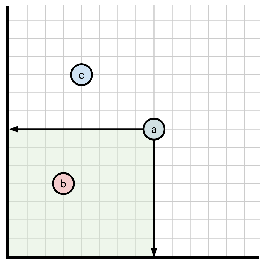
Partially ordered sets are a very rich topic and there are many different examples of them, but for the purposes of reasoning about them in this context I generally visualize the following partially ordered set:

A timestamp is a pair \((x, y)\) of natural numbers. \((x_1, y_1) \le (x_2, y_2)\) if and only if \(x_1 \le y_1\) and \(x_2 \le y_2\).

For example,

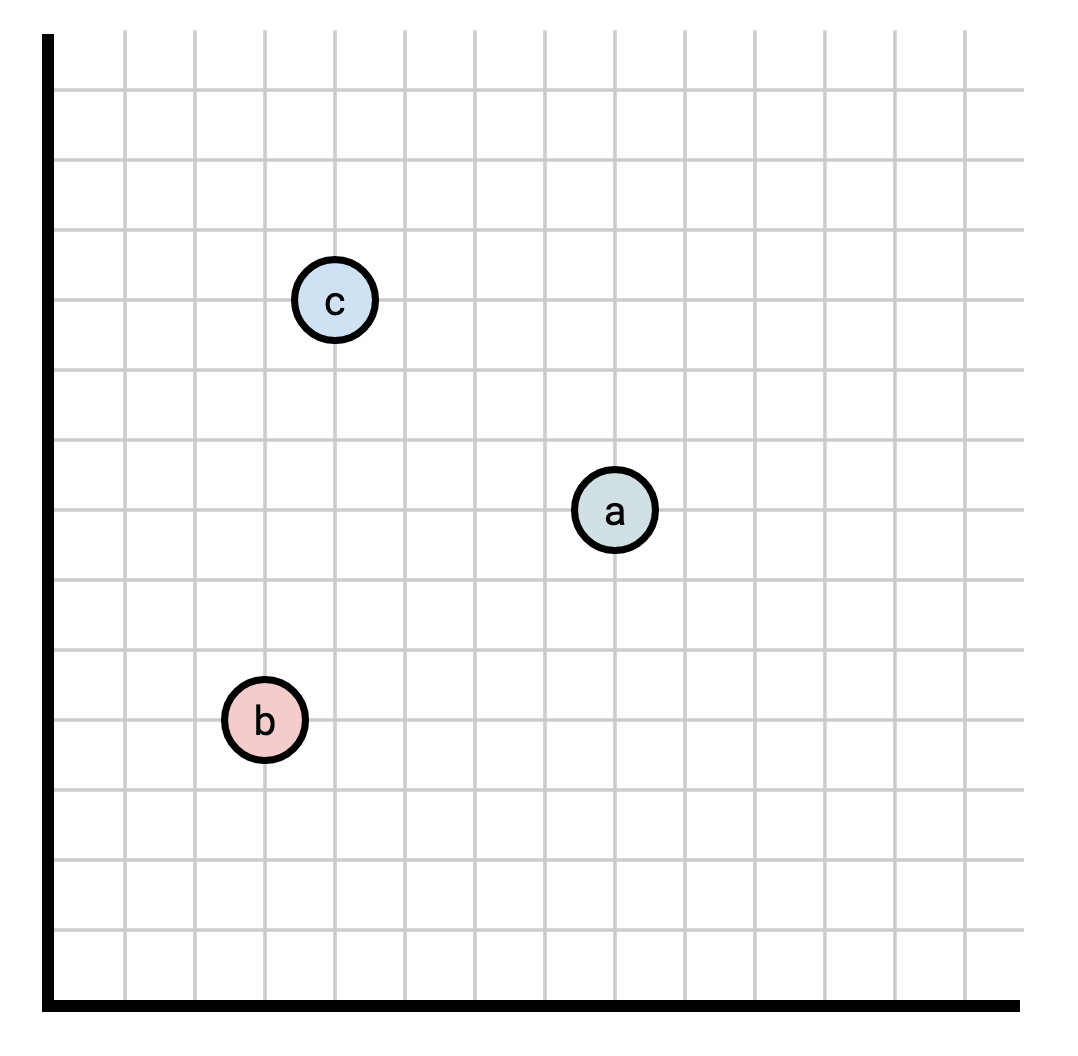
In this diagram, the following relationships are true:

• \(b \le a\) (\(b\) “comes before” \(a\)),
• \(b \le c\) (\(b\) “comes before” \(c\)),
• \(a\) and \(c\) are unrelated (neither “comes before” the other).

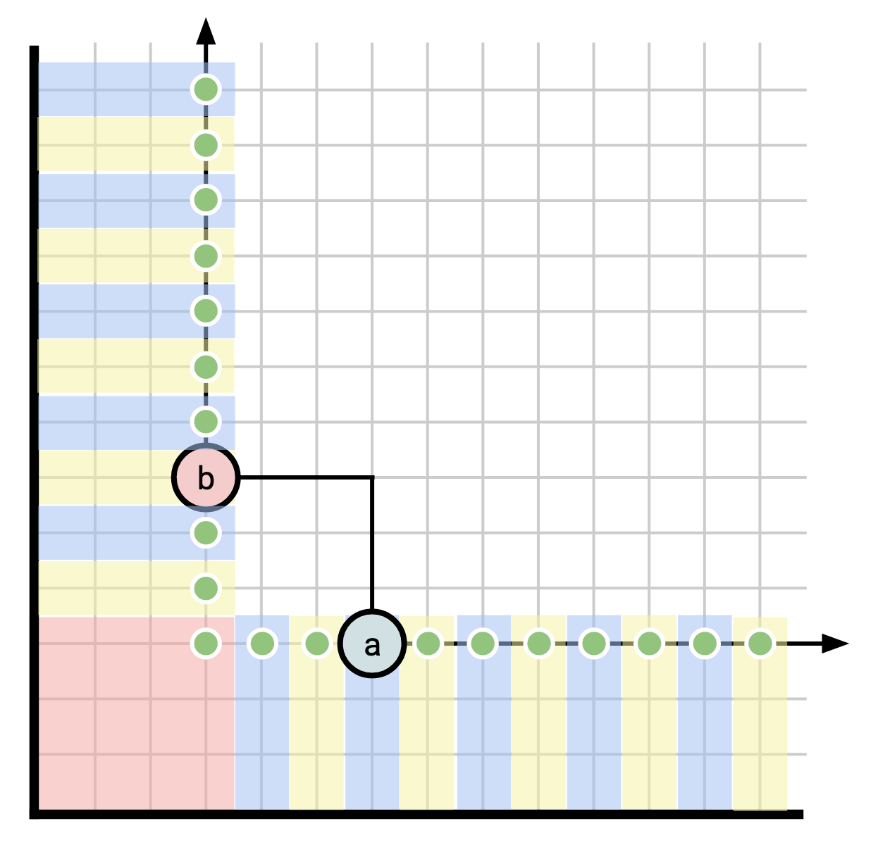
Visually, for two points \(u\) and \(v\), \(u \le v\) if \(u\) falls inside the rectangle having the x- and y-axes as two sides and having \(v\) as one of its corners:

As before, when we read at a timestamp \(t\), we stand atop \(t\) and look backwards to see event on the timeline that “comes before” \(t\). Whereas before, this meant we go backwards along a linear timeline:

Now it means we observe everything inside of our rectangle:

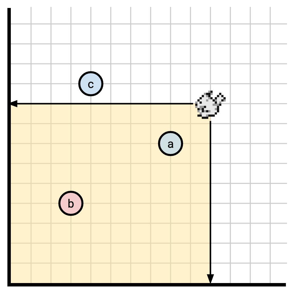
In this diagram, our observer can see a and b. Since we no longer have an obvious order to apply effects in, Differential generally requires that the way we combine events be commutative (meaning that the order we do it in doesn’t matter), so it will generally be things like the multiplicity of a row in a relation. This makes it a bit tricky to do things like key-value semantics sometimes.

The Differential Dataflow paper captures this idea that the state of a collection \(\mathbf A\) at a particular time \(t\) can be computed as the sum of all events ("\(\delta\)“s) at each timestamp occurring before or at \(t\) with the following equation:

$$\mathbf A_t = \sum_{s \le t} \delta \mathbf A_s$$

Differential has the same problem as Pebble: events come in bearing a timestamp, and it would require prohibitive space to maintain fidelity across all of time. It needs a strategy to limit what readers can see that allows it to save space.

Differential doesn’t use snapshots, as Pebble does. The tool Differential uses to express “you may read at some time” is called a frontier. This is a token which corresponds to a set \(F\) of timestamps, which grants the ability to read at any timestamp which is \(\ge\) some \(f \in F\). This creates a region you are allowed to read from that looks like this if \(F = \{a, b, c\}\):

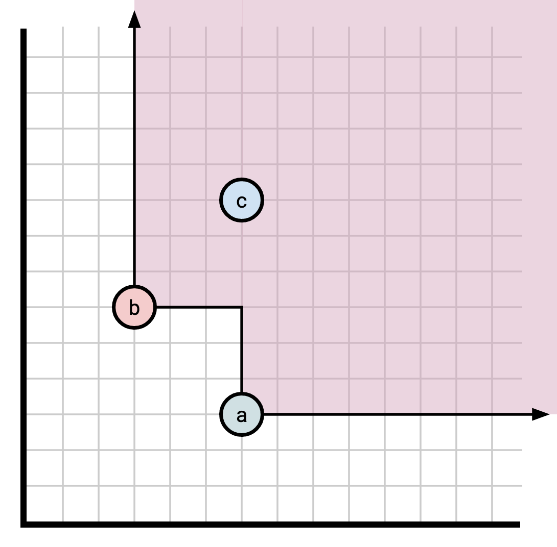
Readers may read at any point in the purple region.

Since \(c \ge a\), \(c\) doesn’t add any extra information to \(F\) (by transitivity, if a point is \(\ge c\), it’s also \(\ge a\)). We can throw away all points except the smallest and retain all the same information. Doing this leaves us with a set of points, all of which are incomparable with each other (this is called an Antichain): \(\{a, b\}\). It might take a bit of thought to convince yourself that this can be done canonically, so draw some pictures if it helps you.

So we have our set of events: the timestamps in this space, and our vantage point: the set of points \(\ge\) some \(f \in F\). We just need to figure out how to compress our events to a logically equivalent form.

The way Differential solves this problem is explained in the paper K-Pg: Shared State in Differential Dataflows.

As before, we need to figure out:

1. When two points are indistinguishable, and
2. how to compute a selector.

Let’s start with an example. Consider the following set of timestamps, with \(a\) and \(b\) comprising our frontier. Try to figure out which timestamps are indistinguishable here.

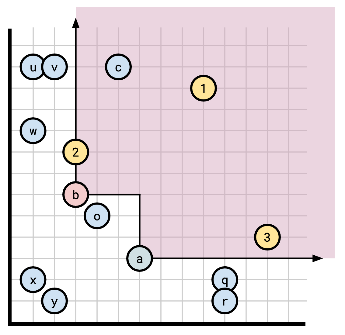
In this diagram:

• \(u\) and \(v\) are indistinguishable,
• \(q\) and \(r\) are indistinguishable, and
• \(x\) and \(y\) are indistinguishable.

All other points are distinguishable. For instance:

• \(1\) distinguishes \(u\) from \(w\),
• \(2\) distinguishes \(o\) from \(x\),
• \(3\) distinguishes \(c\) from \(q\).

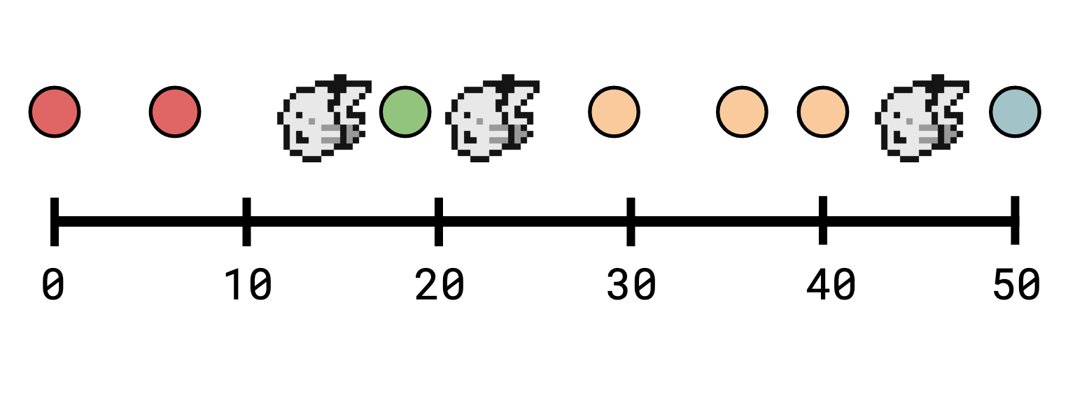
In computing a selector, we want to bring each point to a representative element. Approximately what we’re trying to do is to collapse each equivalence class down to a single point. If we colour in our various equivalence classes, they look something like this.

Each stripe is its own equivalence class, the red region in the bottom left is its own equivalence class, and every other point is a singleton equivalence class. The ideal (latest) representative element for each class is marked in green.

The K-Pg paper provides an algorithm for computing \(\text{rep}\).

Given two times \(a\) and \(b\), the least upper bound (lub) of \(a\) and \(b\) is the smallest point in time where both \(a\) and \(b\) are observable, and is written \(a \vee b\). Likewise, the greatest lower bound (glb) of \(a\) and \(b\) is the latest point in time which \(a\) and \(b\) can both observe, and is written \(a \wedge b\) (note that the K-Pg paper writes these the other way around).

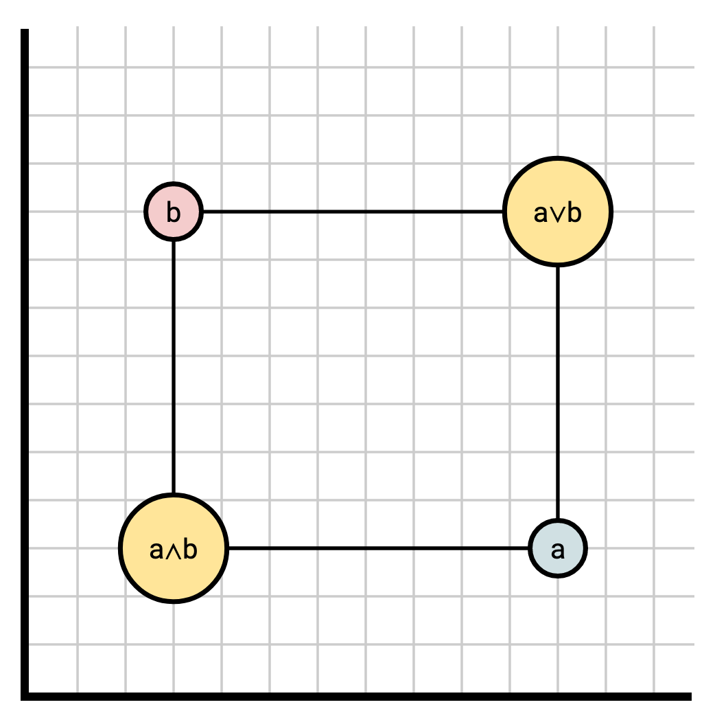
For any timestamp \(t\) and frontier \(F\):

$$ \text{rep}_F(t) = \bigwedge_{f \in F}\left( t \vee f \right) $$

In other words, to find \(\text{rep}_F(t)\), take the lub of \(t\) with each element of \(F\), then take the glb of each of those.

The appendices of the K-Pg paper go into more detail about this, including proofs of correctness.

Comparison

Both systems outlined here do things the other doesn’t: Pebble supports maintaining a single observer arbitrarily far back in time, while the rest of the system can happily advance and compact things that come after it. Differential, on the other hand, is chiefly concerned with the farthest back points, and will never compact data that comes after a possible observer. Giving this up gives it the flexibility to support partially ordered times.

Conclusion

The reason you hear so much about logs in the context of databases is that there’s no more faithful representation of a sequence of events than a precise history of what those events were and when they occurred. Such a representation can become large and unwieldy, and so a tool for simplifying and throwing away resolution we no longer need is important. This tool is compaction.

Compaction is an important part of any system dealing with a nontrivial amount of changing data. To keep strong abstractions, the prime consideration is the vantage point users of the system assume. What can they see and how can you change things out from under them without them noticing? Pebble uses a system that requires total ordering, but allows for compacting points in between observers. Differential Dataflow does not allow compacting points between observers, but in exchange has a much more flexible notion of “timestamp” that does not require total ordering.

Acknowledgements

Bilal Akhtar for explaining Pebble’s compaction, Frank McSherry for explaining Differential’s compaction.