Branch and Bound
11 Jun 2020Sometimes I write posts because I think I have a fresh perspective on something, and sometimes I write posts because for whatever reason I think every explanation of a particular concept that I’ve seen is bad. This is the latter! This post is about a lovely technique for discrete optimization called Branch and Bound.
Optimization problems can generally be viewed as a search for an object with the lowest “cost.” For instance, given an instance of the Traveling Salesman Problem (TSP), the “objects” we’re searching for are “tours,” or a cycle in the graph that visits every “city” exactly once. Of the set of all tours, we are interested in finding the “shortest” (or cheapest perhaps, more generally). The TSP is, famously, NP-hard, and in fact, is probably the most famous of all NP-hard problems.
Let us establish a shared mental model that is not necessarily valid but is useful. If someone tells you an optimization problem you are facing is NP-hard1, what they’re really telling you is that any solution to that problem resembles “check every possible solution and take the best one.”
It might not be realized exactly as that, for instance, dynamic programming is a way to exploit the principle of optimality to kind of inspect every solution. Having something like the principle of optimality lets us sneak around and exploit some structure in order to inspect every solution in a somewhat smarter way (but we’re still fundamentally inspecting every solution). Exploiting this for the TSP brings its complexity from \(O(n!)\) to \(O(n^22^n)\).
Since we’re thinking of this as a “check every solution” kind of problem, let’s visualize the space of all solutions:
The optimal solution is hiding in this space somewhere, we don’t know where, but since there’s a finite set of solutions, there has to be a best one (or several tied for the best, but for simplicity lets assume there’s just one). Now, if we split this up into two (or more) parts, say \(A\) and \(B\):
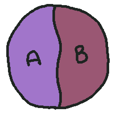
Our solution still lives in this entire space, and it lives in either \(A\) or \(B\), and we can solve each of those subsets of solutions independently and report the best of each of them as our overall “best” solution. Typically we’d partition the space like this in some meaningful way, rather than arbitrarily. If we have an instance of the TSP, for instance, we might say “\(A\) is all the solutions that use the edge \(e\)” and “\(B\) is all the solutions that do not use the edge \(e\).” It’s pretty easy to see this partitions the space: every solution falls into one of those two buckets. We might visualize this dichotomy as a tree:
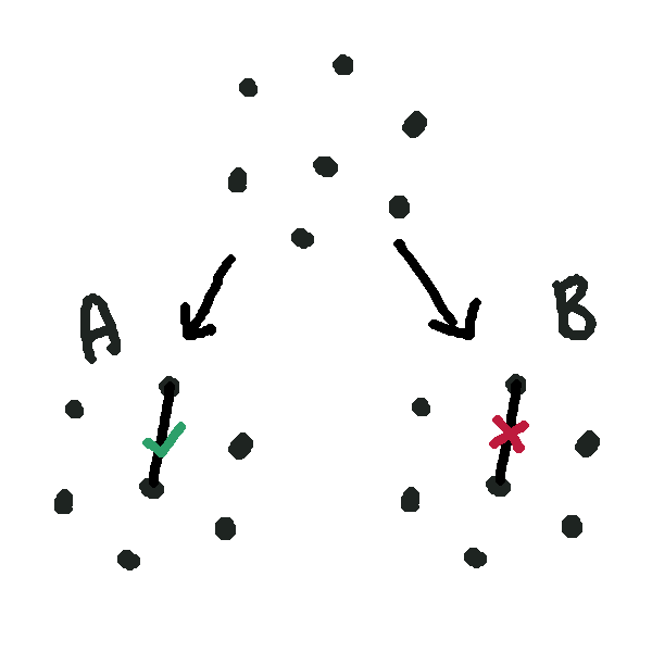
As we recursively subdivide our space like this, we’ll eventually end up with partitions so restricted that they only contain 0 or 1 solutions (or, more realistically, with a set of solutions small enough that we can just solve them by brute force). This is the eponymous “branch.”
This is not that exciting on its own. It’s like, pretty tautological, in the purest sense: “in an optimal solution, \(p\) or not \(p\) for any \(p\),” how exciting. If we grant ourselves a little extra power, we can make use of it, though.
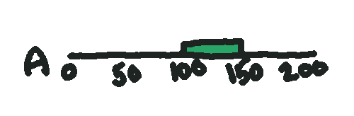
Say we had a magic wand that could give us a range of values that the optimal solution might fall in for one of these branches. We point it at the set \(A\) and it says “oh yeah, you definitely can’t do better than 100 miles if you include that edge. You can definitely do better than 150 miles, though.” It doesn’t know the exact solution, but it can quickly find an upper and lower bound.
Say we next point our magic wand at \(B\), and for whatever reason, it gives us the much less confident range \([50, 200]\).
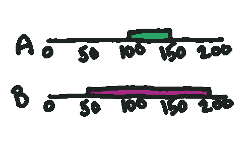
From this, what can we say about the optimal solution overall? We know it has to be more than 50, since our wand tells us neither path has a better outcome than that (and remember, these two paths enumerate every solution). And we know it has to be less than 150, since \(A\) definitely has a solution better than 150.
What if instead we waved our magic wand and saw this outcome instead?
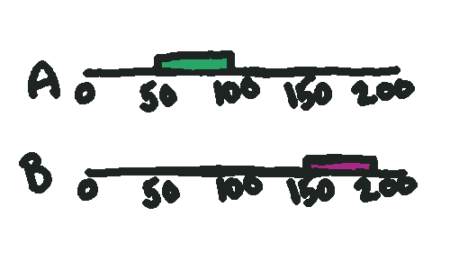
We know \(A\)’s optimal solution is in \([50,100]\) and \(B\)’s is in \([150, 200]\). Since we know that in the absolute worst case, the best solution we’ll get out of \(A\) is 100, and in the absolute best case, the best solution we’ll get out of \(B\) is 150, \(B\) can never contain the optimal solution. If \(B\)’s lower bound is greater than \(A\)’s upper bound, the optimal solution must live in the left half of this diagram.
This means we can completely avoid searching \(B\)!
Our magic wand is the so-called “bound,” and the specific techniques you might use to come up with bounds will vary, but in the case of the TSP,
- you might use a heuristic algorithm like greedy search to find an upper bound,
- and you might find an easier-to-compute object, like a minimum spanning tree (MST), to find a lower bound
The MST works as a lower bound since a MST of a graph is always shorter than a shortest tour (convince yourself of this as an exercise!), and it’s quick to compute since MSTs are just really really easy to find. In fact, you can just like, do the first, most obvious possible thing you can think of and it will probably successfully compute a MST.
It’s also common to use linear programming to find a lower bound, but that’s a bigger topic than this post.
Branch and bound is one of my favourite algorithms because it’s a member of a class that I struggle to define exactly, but I would describe as roughly “makes intuitive ideas precise.” I don’t want you to come away from this thinking this is some magical symbolic trick we’re pulling to create new information out of thin air. The inferences branch and bound lets us make are often “obvious,” in the sense that, if you looked at a problem, you could probably spot them intuitively (and then lament that you were not sure how to translate that intuition into a computer program).
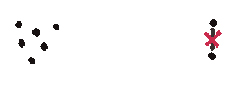
Consider the following instance of the TSP:
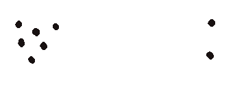
You can probably look at this and immediately recognize that in any optimal tour, those two cities on the right are most likely connected directly to each other. I bet you can convince yourself of that quite easily, in fact. But for a computer to make that judgment we need something more concrete.
For this, we can use branch and bound, and, again, I hope you’ll appreciate that this is really just making explicit what your intuition was already able to tell you.
So first, let’s branch. Here’s case \(A\), where we do take the edge.
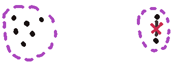
And here’s case \(B\), where we don’t take the edge.
We can find a low-effort upper bound for \(A\) pretty easily, any solution at all suffices as one (if we have an arbitrary solution with cost \(c\), certainly no optimal solution can cost more than \(c\)). There are lots of heuristic algorithms for solving the TSP suboptimally. I’m just gonna sketch out the first solution I see.
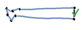
Let’s say this solution has cost 50, so we have an upper bound for taking the edge of 50.
Lower bounding \(B\) is a is a little harder. First, note that we have two “clusters” of cities:
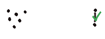
And since we can’t travel between the two cities in the right cluster, any tour has to travel between these two clusters twice: to the upper city and back, and to the lower city and back. This means it has to cross this gulf no less than four times:
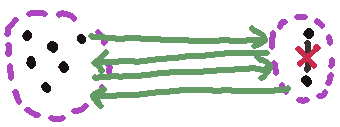
If the gulf is, say, 15 units long, that’s our entire bound right there, we cannot do a tour that does not use this edge for less than 60 units. And so we’re done, we have a lower bound on this branch that’s greater than the upper bound on our other branch, so any optimal tour must include that edge.
If you think this stuff is cool, I recommend the book In Pursuit of the Traveling Salesman by Bill Cook, who taught the class I learned about this in.
1. assuming P!=NP2
2. and come on, P!=NP, we all know it, it's just that nobody is brave enough to say it3
3. do not contact me about this statement