An Introduction to Join Ordering
23 Oct 2018This post was originally posted on the Cockroach Labs Blog
The development of the relational model heralded a big step forward for the world of databases. The introduction of SQL meant that analysts could construct a new report without having to interact with those eggheads in engineering, but more importantly, the existence of complex join queries meant that theoreticians had an interesting new NP-complete problem to fawn over for the next five decades.
Ever since, the join has been the fundamental operation by which complex queries are constructed out of simpler “relations”. Let’s do a quick refresher in case you don’t work with SQL databases on a regular basis. A relation or table is basically a spreadsheet. Say we have the following relations describing a simple retailer:
The customers, or \(C\) relation looks something like this:
| customer_id | customer_name | customer_location |
|---|---|---|
| 1 | Joseph | Norwalk, CA, USA |
| 2 | Adam | Gothenburg, Sweden |
| 3 | William | Stockholm, Sweden |
| 4 | Kevin | Raleigh, NC, USA |
| … | … |
the products, or \(P\) relation looks like this:
| product_id | product_location |
|---|---|
| 123 | Norwalk, CA, USA |
| 789 | Stockholm, Sweden |
| 135 | Toronto, ON, Canada |
| … | … |
the orders, or \(O\) relation looks like this:
| order_id | order_product_id | order_customer_id | order_active |
|---|---|---|---|
| 1 | 123 | 3 | false |
| 2 | 789 | 1 | true |
| 3 | 135 | 2 | true |
| … | … | … |
The cross product of the two relations, written \(P \times O\), is a new relation which contains every pair of rows from the two input relations. Here’s what \(P \times O\) looks like:
| product_id | product_location | order_id | order_product_id | order_customer_id | order_active |
|---|---|---|---|---|---|
| 123 | Norwalk, CA, USA | 1 | 123 | 3 | false |
| 123 | Norwalk, CA, USA | 2 | 789 | 1 | true |
| 123 | Norwalk, CA, USA | 3 | 135 | 2 | true |
| 789 | Stockholm, Sweden | 1 | 123 | 3 | false |
| 789 | Stockholm, Sweden | 2 | 789 | 1 | true |
| 789 | Stockholm, Sweden | 3 | 135 | 2 | true |
| 135 | Toronto, ON, Canada | 1 | 123 | 3 | false |
| 135 | Toronto, ON, Canada | 2 | 789 | 1 | true |
| 135 | Toronto, ON, Canada | 3 | 135 | 2 | true |
| … | … | … | … | … | … |
and a join is when we have a filter (or predicate) applied to the cross product of two relations. If we filter the above table to where the rows where product_id = order_product_id, we say we’re “joining \(P\) and \(O\) on product_id = order_product_id". By itself the cross product doesn’t represent anything interesting, but by filtering like this we can create a meaningful query. The result looks like this:
| product_id | product_location | order_id | order_product_id | order_customer_id | order_active |
|---|---|---|---|---|---|
| 123 | Norwalk, CA, USA | 1 | 123 | 3 | false |
| 789 | Stockholm, Sweden | 2 | 789 | 1 | true |
| 135 | Toronto, ON, Canada | 3 | 135 | 2 | true |
| … | … | … | … | .. | … |
For our final result we only care about some of these fields, so we can then remove some of the columns from the output (this is called projection):
| product_id | order_customer_id |
|---|---|
| 123 | 3 |
| 789 | 1 |
| 135 | 2 |
| … | … |
and we end up with a relation describing the products various users ordered. With pretty basic operations we built up some nontrivial meaning. This is why joins are such a major part of most query languages (primarily SQL): they’re very conceptually simple (a predicate applied to the cross product) but can express fairly complex operations. A real-world query might then join this resulting table with one or more other tables.
Computing Joins
Even though the size of the cross product was quite large (\(|P| \times |O|\)), the final output was pretty small. Databases will exploit that fact to perform joins much more efficiently than by producing the entire cross product and then filtering it. This is part of why it’s often useful to think of a join as a single unit, rather than two composed operations.
To make things easier to write, we’re going to introduce a little bit of notation.
We already saw that the cross product of \(A\) and \(B\) is written \(A \times B\). Filtering a relation \(R\) on a predicate \(p\) is written \(\sigma_p(R)\). That is, \(\sigma_p(R)\) is the relation with every row of \(R\) for which \(p\) is true, for example, the rows where product_id = order_product_id. Thus a join of \(A\) and \(B\) on \(p\) could be written \(\sigma_p(A \times B)\). Since we often like to think of joins as single cohesive units, we can also write this as \(A \Join_p B\).
The columns in a relation don’t need to have any particular order (we only care about their names), so we can take the cross product in any order. \(A \times B = B \times A\), and further, \(A \Join_p B = B \Join_p A\). You might know this as the commutative property. Joins are commutative.
We can “pull up” a filter through a cross product: \(\sigma_p(A) \times B = \sigma_p(A \times B)\). It doesn’t matter if we do the filtering before or after the product is taken. Because of this, it sometimes makes sense to think of a sequence of joins as a sequence of cross products which we filter at the very end: \((A \Join_p B) \Join_q C = \sigma_q(\sigma_p(A \times B) \times C) = \sigma_{p\wedge q}(A \times B \times C)\). Something that becomes clear when written in this form is that we can join \(A\) with \(B\) and then join the result of that with \(C\), or we can join \(B\) with \(C\) and then join the result of that with \(A\). The order in which we apply those joins doesn’t matter, as long as all the filtering happens at some point. You might recognize this as the **associative property**. Joins are **associative**, with the asterisk that we need to move around predicates where appropriate (since some predicates might require information about multiple tables).
Using Commutativity and Associativity
So we can perform our joins in any order we please. This raises a question: is there some order that’s more preferable than another? Yes. It turns out that the order in which we perform our joins can result in dramatically different amounts of work required. Consider a fairly natural query on the above relations, where we want to get a list of all customers’ names along with the location of each product they’ve ordered. In SQL we could write such a query like this:
SELECT customer_name, product_location FROM
  orders
  JOIN customers ON customer_id = order_customer_id
  JOIN products ON product_id = order_product_id
We have two predicates:
customer_id = order_customer_idandproduct_id = order_product_id.
So say we were to first join products and customers. Since neither of the two predicates above relate products with customers, we have no choice but to form the entire cross products between them. This cross product might be very large (the number of customers times the number of products) and we have to compute the entire thing.
Say we instead first compute the join between orders and customers. The sub-join of orders joined with customers only has an entry for every order placed by a customer - probably much smaller than every pair of customer and product. Since we have a predicate between these two, we can compute the much smaller result of joining them and filtering directly (there are many algorithms to do this efficiently, the three most common being the hash join, merge join, and nested-loop join).
In this example there were only a handful of options, but as the number of tables being joined, the number of options grows exponentially, and in fact, finding the optimal order in which to join a set of tables is NP-hard. This means that when faced with large join ordering problems, databases are generally forced to resort to a collection of heuristics to attempt to find a good execution plan (unless they want to spend more time optimizing than executing!).
Finding a Good Join Order
I think it’s important to first answer the question of why we need to do this at all. Even if some join orderings are orders of magnitude better than others, why can’t we just find a good order once and then use that in the future? Why does a piece of software like a database concerned with going fast need to solve an NP-hard problem every time it receives a query? It’s a fair question, and there’s probably interesting research to be done in sharing optimization work across queries. The main answer, though, is that you’re going to want different join strategies for a query involving Justin Bieber’s twitter followers versus mine. The scale of various relations being joined will vary dramatically depending on the query parameters and the fact is that we just don’t know the problem we’re solving until we receive the query from the user, at which point the query optimizer will need to consult its statistics to make informed guesses about what join strategies will be good. Since these statistics will be different for a query over Bieber’s followers, the decisions the optimizer ends up making will be different and we probably won’t be able to reuse a result from before.
A common characteristic of NP-hard problems is that they’re strikingly non-local. Any type of local reasoning or optimization you attempt to apply to them is often doomed. In the case of join ordering, what this means is that in most cases it’s difficult or impossible to make conclusive statements about how any given pair of relations should be joined - the answer differs drastically depending on all the tables you don’t happen to be thinking about at this moment.
In our example with customers, orders, and products, it might look like our first plan was bad only because we first performed a join for which we had no predicate (such intermediate joins are just referred to as cross products), but in fact, there are joins for which the ordering that gives the smallest overall cost involves a cross product (exercise for the reader: find one).
Despite the fact that optimal plans can contain cross products, it’s very common for query optimizers to assume their inclusion won’t improve the quality of query plans that much, since disallowing them makes the space of query plans much smaller and can make finding decent plans much quicker. This assumption is sometimes called the connectivity heuristic.
Genres of Queries
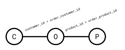
To better understand the structure of a join query, we can look at its query graph. The query graph of a query has a vertex for each relation being joined and an edge between any two relations for which there is a predicate.
Since a predicate filters the result of the cross product, predicates can be given a value that describes how much they filter said result. This value is called their selectivity. The selectivity of a predicate \(p\) on \(A\) and \(B\) is defined as
$$sel(p) = \dfrac{|A \Join_p B|}{|A \times B|} = \dfrac{|A \Join_p B|}{|A||B|}$$
In practice, we tend to think about this the other way around - we assume that we can estimate the selectivity of a predicate somehow and use that to estimate the size of a join:
$$|A \Join_p B| = sel(p)|A||B|$$
So a predicate which filters out half of the rows has selectivity \(0.5\), a predicate which only allows one row out of every hundred has selectivity \(0.01\). Since predicates which are more selective reduce the cardinality of their output more aggressively, a decent general principle is that we want to perform joins over predicates which are very selective first. It’s often assumed for convenience that all the selectivities are independent, that is,
$$|A \Join_p B \Join_q C| = sel(p)sel(q)|A \times B \times C|$$
Which, while convenient, is rarely an accurate assumption in practice. Check out “How Good Are Query Optimizers, Really?” by Leis et al. for a detailed discussion of the problems with this assumption.
It turns out that the shape of a query graph plays a large part in how difficult it is to optimize a query. There are a handful of canonical archetypes of query graph “shapes”, all with different optimization characteristics.

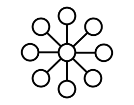
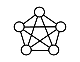
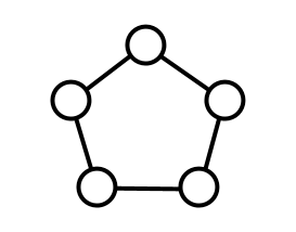
Note that these shapes aren’t necessarily representative of many real queries, but they represent extremes which exhibit interesting behaviour and for which statements can be made.
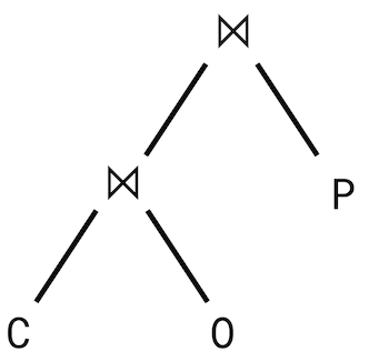
The query plan we ended up with for the above query looks something like this:
There are also two main canonical query plan shapes, the less general “left-deep plan”:
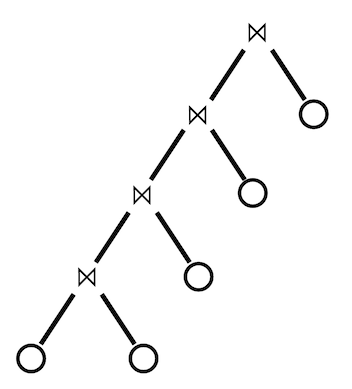
Where every relation is joined in sequence.
The more general form is the “bushy plan”:
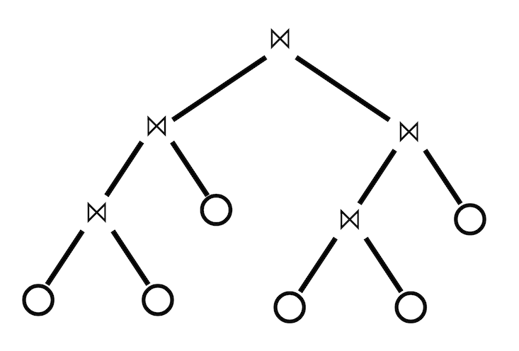
In a left-deep plan, one of the two relations being joined must always be a concrete table, rather than the output of a join. In a bushy plan, such composite inners are permitted.
In the general case (and in fact, almost every more specific case) the problem of finding the optimal order in which to perform a join query is NP-complete. There are a handful of scenarios which permit a more efficient solution, one important one of which I will get into in a followup post.