Functional Dependencies and Orders
25 Dec 2022Say you’re a query optimizer. Is the following transformation “valid?”
select * from t where x > 5
=>
select * from t where false
Well…I doubt it. The first version permits strictly more rows than the second.
But, what if I told you that we recently collected statistics on our data, and found that
no more than 0.01% of our data has a value of x that’s larger than 5?
Well, again, I doubt you’d want to perform this transformation. I’d guess that those 0.01% of rows are precisely the ones whoever is running this query is interested in.
What if I told you that we recently collected statistics on our data, and found that
none of our data has a value of x that’s larger than 5?
Now we’re getting tempting! But the imperative word there is “recently.” Perhaps, since you collected those statistics, a whole lot of data got ingested and they’re now wildly out of date!
Ok, ok.
What if I told you that I recently added a constraint to the table that
rejects rows, old and new, that have a value of x that’s larger than 5?
It sounds like we need a framework.
These scenarios highlight an important question if you want to get philosophical about what your database is doing. What exactly are we saying when we express an optimization rule? When we teach our query optimizer about join commutativity:
(deftransformation
  (join a b p)
  (join b a p))
what does that mean?
A query planner, in some sense, has to balance two competing pressures: first, due to its tight integration with the rest of the database, a planner is expected to generate plans specialized to its user’s data, utilizing information not statically expressed in the schema like table sizes and data distribution. Pushing up against that is the fact that it must always produce plans that are correct, even if the statistical information it’s using to make decisions might be out of date.
In many database architectures, for instance, it would be incorrect to look at statistical information
stating that “the largest value of x in the table t is 5” and optimize
select * from t where x > 5 to select * from t where false,
because said statistical information might not be guaranteed to be consistent.
On the other hand, if there is a constraint on the table requiring x to be no greater than 5,
such an optimization could be valid.
Thus, there is a divide between the types of information a planner can make use of:
- statistical information, like estimated table sizes, histograms, and distinctness counts, and
- static schema information, like column types and integrity constraints.
Which bucket a given piece of information falls into can vary between databases, Snowflake, for instance, keeps certain statistical information consistent, so the planner can rely on it being correct.
In the world of database theory, people are generally concerned with the second kind of information. The machinery we use to talk about database queries formally is to distinguish between a database schema, which describes what data could live in the database, and a database instance, which describes what data does live in the database. This sounds obvious, but I think it’s subtly different from the view that SQL databases push you towards, since they use the same language, SQL, to both modify schemas and to modify data.
The point for me of all this is that this gives us a simple and precise way to talk about when a given query transformation is “valid:” it’s valid for a given schema if it’s valid for every instance of that schema. So even though our queries will always be running against one particular instance, an important correctness condition is that they’re valid for the schema as a whole.
So the answer to what this means:
(deftransformation
  (join a b p)
  (join b a p))
is that we are asserting that these two expressions have the same value for every instance allowed by our schema.
Today, I want to use this machinery to talk about some particularly fun and cool notions pervasive in SQL query optimization.
Ordering Data
Let’s run some SQL queries.
First, I’m going to create a table with a computed column. This is a column whose value is derived from the value of other columns.
$ sqldb
sqldb> create table abc (a int, b int, c int as (b * 2));
Now let’s insert some data into this table.
sqldb> insert into abc (a, b) values
  (1, 2),
  (1, 3),
  (2, 2),
  (2, 3),
  (2, 4),
  (3, 1);
Now let’s read it back. We should see the value of c computed by doubling b:
sqldb> select * from abc;
a|b|c
-+-+-
2|2|4
1|2|4
1|3|6
2|4|8
3|1|2
2|3|6
Note that the rows aren’t arranged in any particular order.
SQL doesn’t guarantee anything about the order of the results in a query,
so if we want the data back in a particular order, we have to use order by:
sqldb> select * from abc order by a;
a|b|c
-+-+-
1|3|6
1|2|4
2|3|6
2|2|4
2|4|8
3|1|2
order by a tells the database we’d like it to retrieve the data ordered on the
a column.
Note, though, that this doesn’t guarantee that the results will always be in the same
order, there’s multiple ways to arrange this result set that are ordered on a.
This response would also have been completely valid:
sqldb> select * from abc order by a;
a|b|c
-+-+-
1|2|4
1|3|6
2|3|6
2|4|8
2|2|4
3|1|2
note that the rows \((1, 2, 4)\) and \((1, 3, 6)\) could have gone in either order, since we’re only comparing by the first coordinate.
If we want to be more precise about the order we want the data, we can specify additional columns:
sqldb> select * from abc order by a, b;
a|b|c
-+-+-
1|2|4
1|3|6
2|2|4
2|3|6
2|4|8
3|1|2
order by a, b is a lexicographic ordering. It means “order first by the a
column, and if two rows have the same value for a, order them by the b column.”
If we wanted to be even more specific, we could order by a, then b, then c:
sqldb> select * from abc order by a, b, c;
a|b|c
-+-+-
1|2|4
1|3|6
2|2|4
2|3|6
2|4|8
3|1|2
But… We might notice that it seems like this doesn’t actually provide any
additional power over just ordering by a, b…
why is that?
We might think this might just be a quirk of the particular data we inserted, this instance,
but it turns out any data we put into this table will have this property.
Thus, it seems as though a clever optimizer might be able to look at a, b, c
and determine that there’s no need for c and eliminate it.
This post will talk a bit about how such determinations can be made.
Let’s get a bit more mathematical and precise.
Orders
A result set is a relation, which is a set of rows, where each column has a name:
id |
pet |
owner |
|---|---|---|
| 1 | Petee | Lauren |
| 2 | Carl | Spencer |
| 3 | Smudge | Justin |
| 4 | Carl | Spencer |
| 5 | Sissel | Justin |
Typically we consider relations to be unordered, since they’re sets. In many contexts, however, we do have an order on them, like if we are streaming them between operators, materializing them in memory, or serializing them to disk. Such an ordering defines a total order \(<_R\) over the rows: \(a <_R b\) if \(a\) comes before \(b\) in \(R\).
If a relation has an ordering upon its rows we call it an ordered relation.
An order is an ordered, distinct list of column names, such as \(\langle \texttt{id} \rangle\), \(\langle \texttt{name} \rangle\), or \(\langle \texttt{name}, \texttt{id} \rangle\).
An order \(O\) defines a preorder \(\le_O\) on the set of rows of a relation: we can compare any two rows lexicographically by comparing their values for the first column in \(O\), then the second, and so on, until we find a place they disagree. If they never disagree, we say they’re peers. Two rows can be peers and not be equal, if they have columns not appearing in the order. This is what makes this a preorder and not a total order: we don’t have antisymmetry unless every column appears in the order.
An ordered relation \(R\) adheres to an order \(O\) if \(\le_R \subseteq \le_O\), or, rather, if \(a\) precedes \(b\) in \(R\), then \(a \le_O b\).
More concretely, if you typed order by c1, ..., cn in a SQL terminal,
the order of the result you get should always adhere to \(\langle c_1, \ldots, c_n \rangle\).
Let’s come up for air and look at some examples. We need the formalism because I want to show some fun stuff about these things, but the ideas are not hard. Let’s consider our relation \(R\) from above:
id |
pet |
owner |
|---|---|---|
| 1 | Petee | Lauren |
| 2 | Carl | Spencer |
| 3 | Smudge | Justin |
| 4 | Carl | Spencer |
| 5 | Sissel | Justin |
As written, this relation adheres to \(\langle \texttt{id} \rangle\) since the
rows are in the order of the id column.
It does not adhere to
\(\langle \texttt{pet}, \texttt{owner} \rangle\). This is because
\[(\text{1}, \text{Petee}, \text{Lauren}) <_R (\text{2}, \text{Carl}, \text{Spencer})\] (because the first row physically
comes before the second),
but
\[
(\text{2}, \text{Carl}, \text{Spencer}) <_{\langle \texttt{pet}, \texttt{owner} \rangle} (\text{1}, \text{Petee}, \text{Lauren})
\] (because “Carl” is alphabetically before “Petee,” and under \(\langle \texttt{pet}, \texttt{owner} \rangle\), the pet column is how we compare rows first).
Since the two disagree somewhere, \(R\) doesn’t adhere to \(\langle \texttt{pet}, \texttt{owner} \rangle\).
Ordering Orders
Orderings can have interesting relationships to each other.
Note that any ordered relation that adheres to
\(\langle \texttt{owner}, \texttt{pet} \rangle\)
also adheres to
\(\langle \texttt{owner} \rangle\), since if something is ordered on owner
and then pet, it must also be ordered on owner.
Intuitively, \(\langle \texttt{owner}, \texttt{pet} \rangle\) is “stronger” than \(\langle \texttt{owner} \rangle\).
This is where we will use our schema/instance distinction to figure out exactly what we mean.
If every instance of a schema adhering to \(P\) also adheres to \(O\), we say \(P\) is as strong as \(O\) and write \[ O \le P. \]
Claim: \(O \le P\) if and only if the columns in \(O\) are a prefix of the columns in \(P\).
Proof:
The case where \(O\) is a prefix of \(P\) is easy: any pair of rows which are \(\le_P\) must clearly also be \(\le_O\) since there is a subset of the comparisons being made, so \(O \le P\).
For the other direction (where \(O\) is not a prefix of \(P\)), we want to show there is some ordered relation \(R\) that adheres to \(P\) but not \(O\), and for that it suffices to find two rows \(r, s\) such that \(r >_O s\) and \(r \le_P s\).
If \(P\) is a prefix of \(O\), there’s some column \(o\) that appears in \(O\) immediately following their shared prefix. Construct \(r\) and \(s\) so that they agree on the shared prefix, and not on that column:
| … | \(o\) | … |
|---|---|---|
| … | 1 | … |
| … | 0 | … |
Now assume \(P\) is not prefix of \(O\). Then there is some pair of columns \(p\) and \(o\) immediately following the common prefix of the two orders.
Again, construct \(r\) and \(s\):
| … | \(o\) | \(p\) | … |
|---|---|---|---|
| … | 1 | 0 | … |
| … | 0 | 1 | … |
For both cases, the constructed rows satisfy \(r >_O s\) and \(r \le_P s\) \(\square\).
Functional Dependencies
A functional dependency is a pair \(X \rightarrow Y\) where \(X\) and \(Y\) are sets of column names.
A result set \(S\) adheres to a set of functional dependencies \(F\) if for every \(X \rightarrow Y \in F\), whenever two rows in \(S\) agree on \(X\), they also agree on \(Y\). Another way to state this is that the projection of \(S\) to \((X, Y)\) is functional (hence the name “functional dependency”).
The closure of a set of functional dependencies \(F^*\) is the set of functional dependencies that can be inferred from \(F\). It can be generated by repeated application of Armstrong’s Axioms:
- Reflexivity: If \(Y \subseteq X\) then \(X \rightarrow Y\).
- Augmentation: If \(X \rightarrow Y\) then \(X\cup Z \rightarrow Y \cup Z\).
- Transitivity: If \(X \rightarrow Y\) and \(Y \rightarrow Z\) then \(X \rightarrow Z\).
See this earlier post for more details.
Functional dependencies are how we will capture the situation we opened with, where we had a column derived from other columns. Note that in any instance of this schema:
sqldb> create table abc (a int, b int, c int as (b * 2));
we must have \[ \{b\} \rightarrow \{c\}. \]
This is somewhat contrived, but functional dependencies arise very naturally in many SQL queries, both simple and complex.
Ordering Orders Pt. 2
Oftentimes when planning a query, we know that a given relation adheres to some set of functional dependencies. Functional dependencies can impact the way that orderings relate to each other. Consider our relation from before:
id |
pet |
owner |
|---|---|---|
| 1 | Petee | Lauren |
| 2 | Carl | Spencer |
| 3 | Smudge | Justin |
| 4 | Carl | Spencer |
| 5 | Sissel | Justin |
While this is just one instance, let’s assume that the following will be true of any instance:
- Every row has a unique
id. This means we have the functional dependency \(\{ \texttt{id} \} \rightarrow \{ \texttt{pet}, \texttt{owner} \} \). - Every pet has a unique
owner, this means we have the functional dependency \(\{ \texttt{pet} \} \rightarrow \{ \texttt{owner} \} \).
(remember that if we were automating this process in a database, we’d need to know statically that these two assumptions would always be true, likely via some kind of integrity constraint.)
If we restrict ourselves to instances that obey those functional dependencies, we can reach some interesting conclusions. Not only do we have \[ \langle \texttt{pet} \rangle \le \langle \texttt{pet}, \texttt{owner} \rangle, \] as before, but, perhaps surprisingly, we have the reverse: \[ \langle \texttt{pet}, \texttt{owner} \rangle \le \langle \texttt{pet} \rangle. \] as well.
You might view this as, “if I can only see how they actually behave in a valid instance, I can’t distinguish between \(\langle \texttt{pet}, \texttt{owner} \rangle\) and \(\langle \texttt{pet} \rangle\).” We care a lot about this kind of indistinguishability in the world of query planning. If a user asks us for a particular order, but we think we can cheaply provide some different order, if it turns out those two orders are actually the same in every instance, we might be able to service their query more efficiently.
Remember what we’re saying here: I’m claiming that any instance that adheres to \( \langle \texttt{pet} \rangle \) also adheres to
\( \langle \texttt{pet}, \texttt{owner} \rangle \).
Why might that be true?
It’s because we have \(\{ \texttt{pet} \} \rightarrow \{ \texttt{owner} \} \),
which means any time two rows agree on pet (precisely when we’d then compare
their owners), they also agree on owner, so no matter what order they’re in,
they can’t be out-of-order.
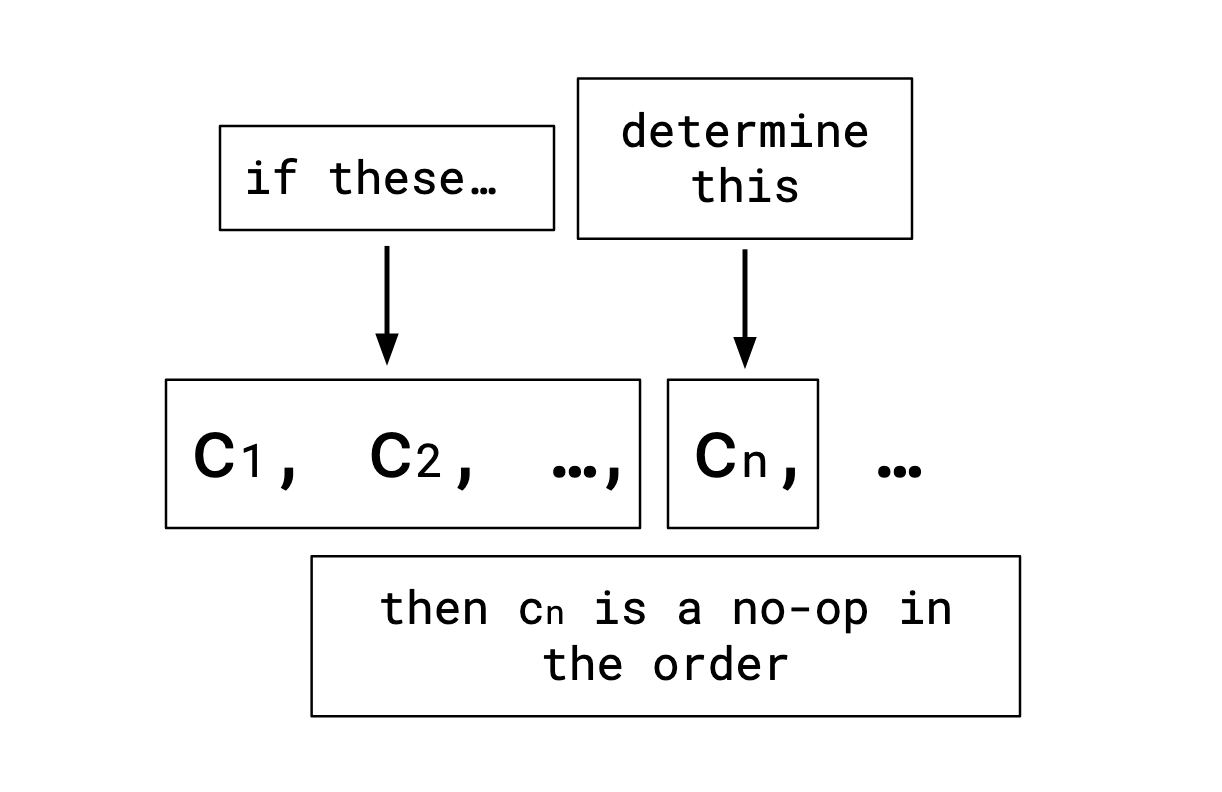
The rough idea is that as we read an order from left-to-right, for any given row we’re accumulating a set of fixed values. If we ever see a column that’s determined by the columns we’ve already seen, that column only has one possible value, and thus is irrelevant to the order.
For a set of functional dependencies \(F\), define a new partial order \(\le_F\) on the set of orderings in more-or-less the same way as before: let \(O\) and \(P\) be orderings. For every instance \(R\) adhering to \(F\), if \(R\) adhering to \(P\) implies \(R\) adheres to \(O\), \(O \le_F P\) (you could call this “strength given adherence to \(F\)").
It would be really nice if we could automate this determination.
If a user were to write select * from t order by pet, owner, and we have an index on pet,
there’s no need to do any sorting, since this is indistinguishable from them writing
select * from t order by pet,
but to actually avoid the sort, we need to be able to detect this.
You might say, “well, why would they write an obviously redundant query?” This is a reasonable objection to have, but a crucial perspective on query optimization is that most queries are not written by humans. It’s important that queries generated by dashboards, ORMs, or other query optimization rules need not be concerned with eliminating such redundancy. That’s the query optimizer’s job.
Ordering Orders with Functional Dependencies
We’d like an easy way to compute \(\le_F\). We can do this via a representative.
Define \(\text{rep}_F(O)\) to be \(O\), but removing any columns which are determined by the columns preceding them in \(O\) according to \(F\).
Algorithmically this would look something like:
def rep(O, F):
  F = F*
  out = []
  fixed_cols = {}
  for col in O:
    if not F.contains(fixed_cols -> col):
      out.push(col)
    fixed_cols.add(col)
  return out
Claim: \(O \le_F P\) if and only if \(\text{rep}_F(O) \le \text{rep}_F(P)\).
Note that if this claim were true it would give us an easy way to evaluate \(\le_F\): simply take the representatives of the two orders and check if the first is a prefix of the second.
Lemma: for all \(O\) and \(F\), \(O \le_F \text{rep}_F(O)\) and \(\text{rep}_F(O) \le_F O\) (meaning they agree on all pairs of rows).
Proof of lemma: if the two disagree on some pair of rows, the disagreement must be in a column present in \(O\) and not \(\text{rep}_F(O)\) or any earlier column in \(O\). Thus, that column was determined by the columns preceding it in \(O\), so two rows agreeing on the preceding columns can never differ on it, a contradiction.
Proof of Claim (forwards direction: \(O \le_F P \rightarrow \text{rep}_F(O) \le \text{rep}_F(P)\)):
By the lemma, and the fact that \(\le_F\) is transitive,
\[ O \le_F P \rightarrow \text{rep}_F(O) \le_F \text{rep}_F(P) \]
Assume \(\text{rep}_F(O) \le_F \text{rep}_F(P)\) and \(\text{rep}_F(O) \not\le \text{rep}_F(P)\).
As we saw earlier, this means that \(\text{rep}_F(O)\) is not a prefix of \(\text{rep}_F(P)\).
We can now repeat the same proof as before:
If \(\text{rep}_F(P)\) is a prefix of \(\text{rep}_F(O)\), them construct these rows, where \(o\) is the first column not appearing in \(\text{rep}_F(P)\):
| … | \(o\) | … |
|---|---|---|
| … | 1 | … |
| … | 0 | … |
and if not, let \(o\) and \(p\) be the first columns that differ in the two, and construct these rows:
| … | \(o\) | \(p\) | … |
|---|---|---|---|
| … | 1 | 0 | … |
| … | 0 | 1 | … |
These rows can be made to be valid even in relations adhering to \(F\), since by the construction of the representatives, neither \(o\) nor \(p\) are determined by the columns in the shared prefix, contradicting \(\text{rep}_F(O) \le_F \text{rep}_F(P)\).
Proof of Claim (reverse direction: \(\text{rep}_F(O) \le \text{rep}_F(P) \rightarrow O \le_F P \)):
By the lemma, and the fact that \(\le\) is transitive,
\[ \begin{aligned} \text{rep}_F(O) &\le \text{rep}_F(P) \rightarrow O \le P \end{aligned} \] since \(\le_F\) considers a subset of relations (namely, it only considers those adhering to \(F\)), it’s weaker than \(\le\), giving \[ \begin{aligned} O &\le_F P \end{aligned} \] as needed \(\square\).
There’s additional dependencies that can give rise to even more equivalencies: whether two columns are always equal (which can be common following a join), whether one column to another is a monotonic function (which can be common in cases like extracting the month from a date), etc.
This is of course a small piece of what makes up a query optimizer. Things like orders, partitions, and functional dependencies make up the vocabulary of how optimizers think about relations, and I think it’s important to have a solid foundation to build more complex optimizations on top of.
Thanks to my friend Ilia for help sorting out this post.