A Gentle(-ish) Introduction to Worst-Case Optimal Joins
30 May 2022If you’ve been following databases in the past couple years, you’ve probably encountered the term “worst-case optimal joins.” These are supposedly a big deal, since joins have been studied for a long time, and the prospect of a big shift in the way they’re thought about is very exciting to a lot of people.
The literature around them, however, is primiarly aimed at theorists. This post is as gentle and bottom-up as I can manage of an introduction to the main ideas behind them. I am decidedly not a theorist, so much of this is probably oversimplified, but I hope the perspective of someone whose background is in traditional query processing can provide some useful insight to people outside the sphere of researchers working on this stuff.
A relation is a set of column names combined with a set of rows, where each row has a value for each column name.
This is a relation \(R\) with three rows, whose column names are \(\{\texttt{a}, \texttt{b}\}\).
| \(\texttt a\) | \(\texttt b\) |
|---|---|
| 1 | 2 |
| 3 | 2 |
| 1 | 3 |
This is a relation \(S\) with four rows, whose column names are \(\{\texttt{b}, \texttt{c}\}\).
| \(\texttt b\) | \(\texttt c\) |
|---|---|
| 2 | 4 |
| 2 | 5 |
| 3 | 6 |
| 3 | 7 |
The join of two relations is computed by taking every pair of rows from the two relations and keeping the ones that agree on all columns with the same name. The join’s column set is the union of the two input column sets.
The join of \(R\) and \(S\), written \(R \bowtie S\), is
| \(\texttt a\) | \(\texttt b\) | \(\texttt c\) |
|---|---|---|
| 1 | 2 | 4 |
| 1 | 2 | 5 |
| 3 | 2 | 4 |
| 3 | 2 | 5 |
| 1 | 3 | 6 |
| 1 | 3 | 7 |
There’s a bunch of equivalent ways to define the join of two relations, but this one will work for us. Joins are nice because they’re a way to algebraically represent the act of “looking things up”: “for each row in side A, look up the corresponding value in side B that has the same column values.”
Here are some useful properties of joins:
- A join is commutative: \(R \bowtie S = S \bowtie R\).
- A join is associative: \((R \bowtie S) \bowtie T = R \bowtie (S \bowtie T)\).
Hopefully you don’t find these too hard to convince yourself of, but try running through some examples if you don’t see why these should be true (remember we don’t care about the order of the columns in a relation).
There’s a natural way to extend the idea of a join to more than two tables: just join them one at a time. Since the operation is commutative and associative (useful properties 1 and 2), it doesn’t matter what order you do this in, the result is well-defined.
A set of tables we wish to join this way is called a join query.
Answering Join Queries
Traditional database systems are typically only able to join two tables at once. Since, as we saw, joins are commutative and associative, this is sufficient for them to be able to answer join queries comprised of many tables: pick your two favourite tables and join them to get an intermediate relation, then join that with another table, and so on, until you’re left with a single table, which is the result of the join query.
We represent this process of joining pairs of tables as a join tree, or query plan.
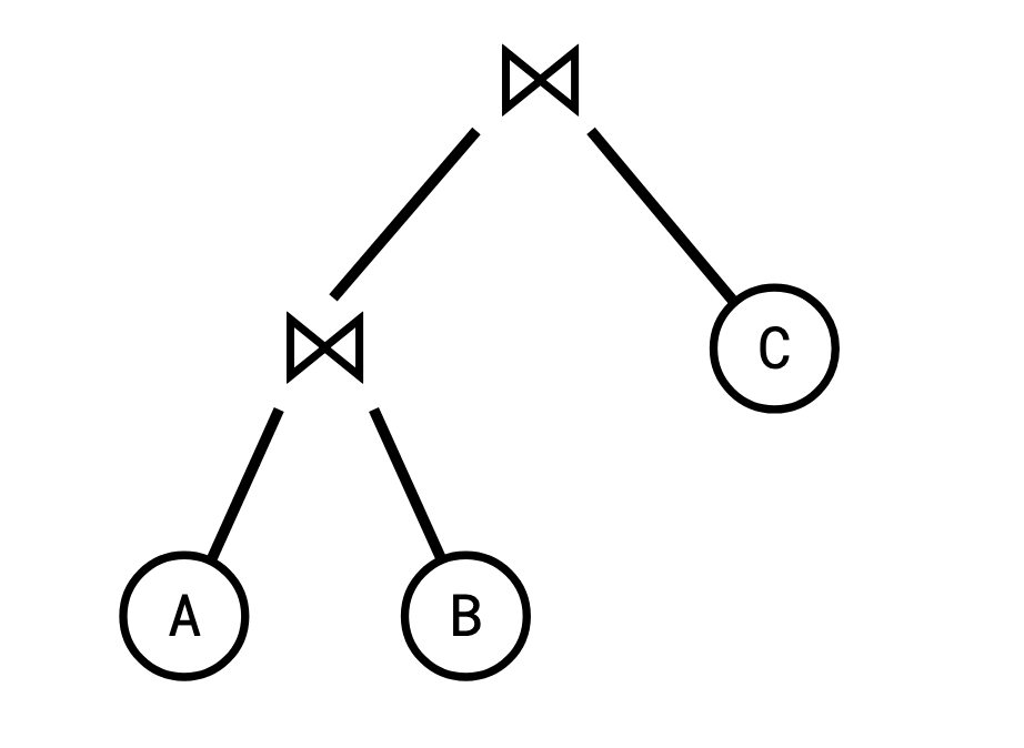
This strategy of computing a join is called binary joins. A well known fact among database people is that not all join trees are created equal. Depending on the size of the intermediate relations, one join tree might be much more efficient to compute than another.
If the intermediate join \(A \bowtie B\) is very large (say, if they had no columns in common), we might compute a lot of rows that will end up getting discarded by the subsequent join with \(C\).
This discrepancy can be seen if we write out a hypothetical size for each possible intermediate join (\(I\) is the join identity, having zero columns and one row):
| Expression | Row Count |
|---|---|
| \(I\) | 1 |
| \(A\) | 100 |
| \(B\) | 1000 |
| \(C\) | 2000 |
| \(A \bowtie B \) | 100000 |
| \(B \bowtie C \) | 10000 |
| \(A \bowtie C \) | 20 |
| \(A \bowtie B \bowtie C \) | 100 |
While not a perfect indicator, this suggests that if we compute the total join by first computing \(A \bowtie C\), rather than \(A \bowtie B\), we’ll probably end up processing fewer rows total.
Much work, both industrial and academic, has been done on the topic of picking the best join tree for a given join query (I myself have written about it twice already).
Joins are Secretly Graph Processing Algorithms
Here’s another perspective on joins: that they’re graph processing algorithms.
Say we had the same relations as before:
\(R\)
| \(\texttt a\) | \(\texttt b\) |
|---|---|
| 1 | 2 |
| 3 | 2 |
| 1 | 3 |
\(S\)
| \(\texttt b\) | \(\texttt c\) |
|---|---|
| 2 | 4 |
| 2 | 5 |
| 3 | 6 |
| 3 | 7 |
We can represent these tables as a graph with three independent sets of vertices:
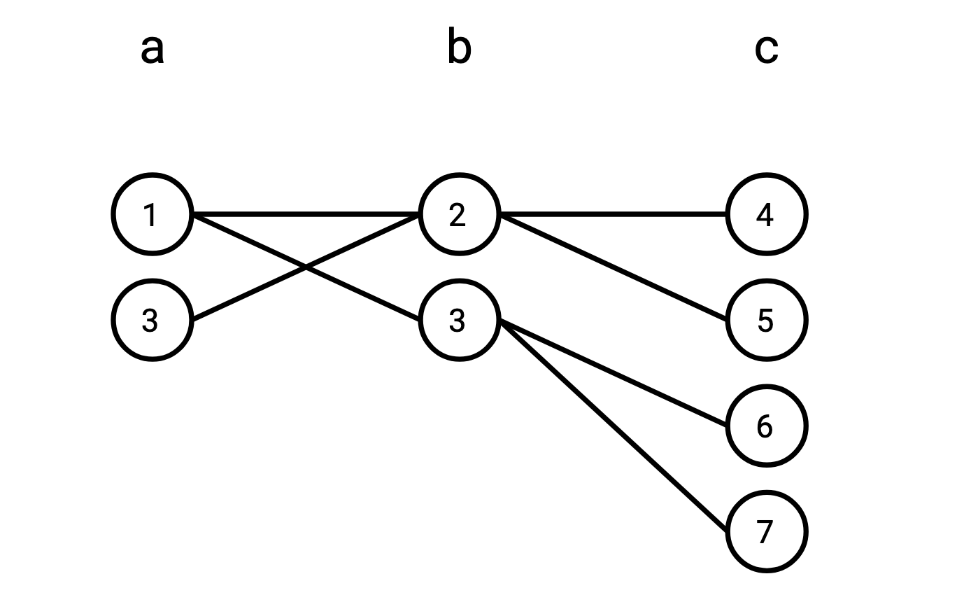
If you enumerate all the paths that start from a vertex in \(\texttt{a}\), go to a vertex in \(\texttt{b}\), and wind up on a vertex in \(\texttt{c}\), you’ll find that set of such paths is precisely \(R \bowtie S\).
What this means is that we can use joins to find structures in graphs.
Say I have the following graph:
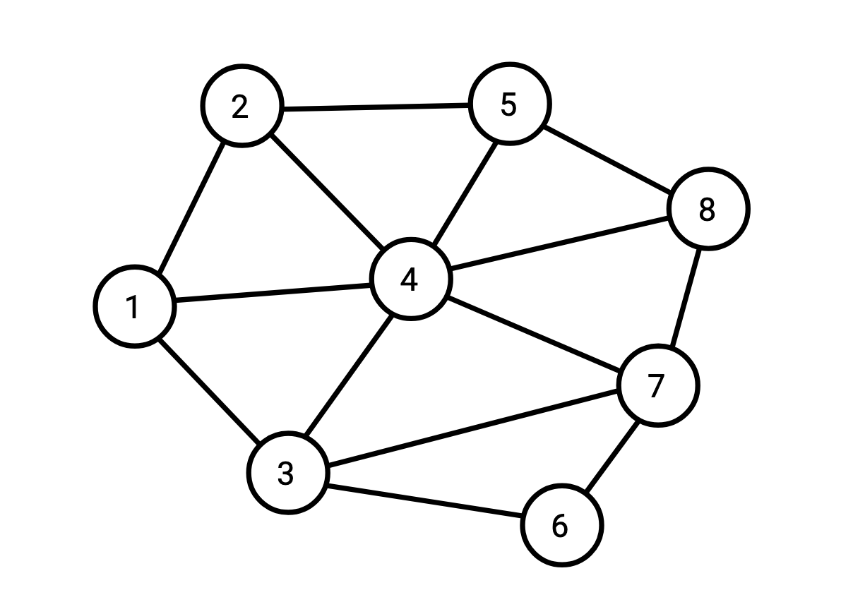
and I want to compute all the triangles (triplets of vertices which are all connected to each other) in this graph.
We can represent this graph as a table containing its edge set:
\(G\)
| \(\texttt{from}\) | \(\texttt{to}\) |
|---|---|
| 1 | 2 |
| 1 | 3 |
| 1 | 4 |
| 2 | 4 |
| 2 | 5 |
| 3 | 4 |
| 3 | 6 |
| 3 | 7 |
| 4 | 5 |
| 4 | 7 |
| 4 | 8 |
| 5 | 8 |
| 6 | 7 |
| 7 | 8 |
Now here’s the clever trick: we can join this table with itself twice, and, if we rename the columns appropriately, out pops the set of triangles.
To prove this trick actually works, here it is in Postgres:
CREATE TABLE g(f INT, t INT);
INSERT INTO g
VALUES
        (1, 2), (1, 3), (1, 4), (2, 4), (2, 5),
        (3, 4), (3, 6), (3, 7), (4, 5), (4, 7),
        (4, 8), (5, 8), (6, 7), (7, 8);
SELECT
    g1.f AS a, g1.t AS b, g2.t AS c
FROM
    g AS g1, g AS g2, g AS g3
WHERE
    g1.t = g2.f AND g2.t = g3.t AND g1.f = g3.f;
to which the answer is:
 a | b | c
---+---+---
 1 | 3 | 4
 1 | 2 | 4
 2 | 4 | 5
 3 | 6 | 7
 3 | 4 | 7
 4 | 7 | 8
 4 | 5 | 8
(7 rows)
Note that we oriented all the edges to point the same direction, from lower numbered vertices to higher, so we don’t need to divide out by any kind of symmetry to get the distinct triangles. You could also include each edge twice, once pointing each direction, and you’d get each triangle six times in the output.
If we look at the query plan for how Postgres computed this result by running it
with EXPLAIN, we see that it used a binary join plan like we talked about
earlier (I cut out a lot of gunk to make this easier to read):
               QUERY PLAN
----------------------------------------
Join ((g2.t = g3.t) AND (g1.f = g3.f))
    ->  Join (g1.t = g2.f)
        ->  Seq Scan on g g1
        ->  Seq Scan on g g2
    ->  Seq Scan on g g3
So it first joins g1 and g2, then joins that with g3.
Now here’s the point of this whole exercise:
- it turns out that a graph with \(n\) edges will have no more than \(O(n^{1.5})\) triangles in it (we’ll see why in a bit).
- there are graphs where that first intermediate join will always have \(O(n^2)\) rows in it, no matter which two tables we choose to join first.
What this means is that for this problem, any binary join strategy will necessarily do more work than the theoretical minimum (where the “theoretical minimum” is “the number of results we might have to emit”) in some cases.
Resolving this issue is the crux of “worst-case optimal joins:” a “worst-case optimal join algorithm” is one that asymptotically does no more work than the maximum number of tuples that could be emitted from a join query.
As it turns out, such algorithms exist and I’ve described one simple one in the appendix of this post. As you might guess, the main idea is that instead of joining two tables at a time (since we’ve seen that approach is doomed), we’re going to join all of the tables at once. For the rest of this post I’d like to focus on something I think is more interesting: what is the worst-case runtime for any given join query?
What is the Theoretical Minimum?
Let’s try to come up with an easy bound on the number of rows a join query can output.
The query graph of a join query has a vertex for every column name and an edge for every relation, and that edge connects all the vertices in that relation (thus, it might be a “hyperedge,” connecting more than two vertices).
Say I’m joining three tables, \(R\), \(S\), and \(T\), whose vertex sets are \(\{\texttt a,\texttt b\}\) for \(R\), \(\{\texttt b,\texttt c\}\) for \(S\), and \(\{\texttt a,\texttt c\}\) for \(T\). The query graph for this query would look like this:
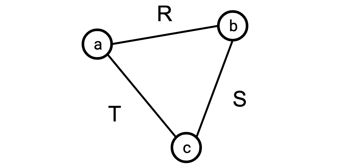
(Observe that if we set \(R = S = T = G\) this is once again our triangle-finding join.)
In additional to the ones from before, let’s note some additional properties of joins:
- The number of rows in a given join (written \(|R \bowtie S|\)) is no larger than the product of the sizes of the two inputs (\(|R||S||\)), since in the worst case, every pair of rows agree on their common columns: \(|R \bowtie S| \le |R||S|\).
- If the column set of \(R\) is a subset of the column set in \(S\), then \(|R \bowtie S| \le |S|\).
The first of these should be pretty easy to convince yourself of. The second one is a little less obvious but still easy: a given row from the table with more columns can match with at most one row in the table with fewer columns (since, unlike in SQL, we’re requiring all of our rows here to be distinct), so the join can only get smaller (because some rows didn’t have a match) or stay the same size (because every row had exactly one match). To convince yourself of this, try joining the examples \(R \bowtie S\) and \(R\) above.
Because of property 3 above, we know the number of rows in \(R \bowtie S \bowtie T\) cannot be larger than \(|R||S||T|\). But actually, we can do a little better. If we join any two relations, say \(R\) and \(S\), that gives us the entire column set: \(R \bowtie S\) has column set \(\{\texttt a, \texttt b,\texttt c\}\). And so by property 4, \(|R \bowtie S \bowtie T| \le |R \bowtie S| \le |R||S|\) (and the same is true for \(|R||T|\) and \(|S||T|\)).
In general, given a join query, once we’ve picked a set of relations that give the entire column set, joining in the remaining relations can only reduce the size of the result due to property 4.
In the language of our query graph, such a set of relations is called an edge covering. We want to choose some set of edges/relations \(E\) such that every vertex is incident to at least one \(e \in E\). If every vertex is adjacent to some relation, we’ve introduced every column to our query. Then, the final size of our join can be no larger than the product of the sizes of the relations we picked (because of property 3).
We can express this symbolically. This symbolic representation is going to look a bit unmotivated at first, but will make more sense when we see how we’re going to generalize it.
If we are joining \(R_1, \ldots, R_n\), define \(x_i\) to be 1 if we picked \(R_i\), and 0 otherwise. This is convenient since we can use \(|R_i|^{x_i}\) to be the size of \(R_i\) if we picked it and 1 otherwise. For some column \(c\), let \(E_c\) be the set of relations that include \(c\).
So. For each \(x_i\) we want \[ x_i \in \{0, 1\} \] (“we either pick a relation, or we don’t”)
Then for each \(c\) we want \[ \sum_{i \in E_c} x_i \ge 1 \] (“each column is present in at least one picked relation”).
Then our bound is \[ |R_1 \bowtie \ldots \bowtie R_n| \le \prod_{i = 1}^n |R_i|^{x_i} \] (“the number of rows in the result is no larger than the product of the sizes of the picked relations”)
This bound is not particularly tight: when applied to our triangle query, it only gets us to the fact that the output is no more than \(n^2\) tuples.
Here’s the thing: there’s a natural but surprising generalization of this bound. If this were a lecture, here’s the part where I would walk over to where I wrote \[ x \in \{0, 1\}, \] erase it, and rewrite \[ x \in [0, 1]. \]
(that is, \(x\) need not be either 0 or 1, but can also be any real number in between) A fractional edge cover is an assignment of values in \([0, 1]\) to each edge in a graph, such that the sum of all weights adjacent to every vertex is at least 1. If instead of finding an edge cover, we relax to allow a fractional edge cover, the bound still holds. That is, we can change our decision for a given relation to be not just “take or not take” but “how much to take.” This, in, theory, should allow us to get a tighter bound, since we now have strictly more options.
And indeed, this change allows us to get to the tight bound of our triangle query. Rather than taking \(x_R = 1, x_S = 1, x_T = 0\), say, we can take \(x_R = \frac12, x_S = \frac12, x_T = \frac12\).
Now \(\texttt{a}\) gets \(\frac12\) weight from each of \(R\) and \(T\), for a total of 1, \(\texttt{b}\) gets it from \(R\) and \(S\), and \(\texttt{c}\) gets it from \(S\) and \(T\).
We’ve still covered every vertex, but now this gives us that \[ |R \bowtie S \bowtie T| \le |R|^{\frac12} |S|^{\frac12} |T|^{\frac12} = \sqrt { |R| |S| |T|}, \]
which, if as before, we set them all equal to our graph \(G\), gives us the \(n^{1.5}\) bound: \[ \sqrt { |R| |S| |T|} = |G|^{1.5} \]
This bound, where we permit a fractional edge cover, is called the AGM Bound, and it holds for any query graph.
Conclusion
I hope this post has made WCOJs a little less scary—it’s very cool to see new research in an area that’s been around for so long.
But what’s the status of the hype? If these things are so great, why haven’t we seen more widespread adoption? Why has there not been a push to get WCOJs into something like Postgres, and why aren’t more vendors loudly advertising their support of them? Well, probably a bunch of confounding factors.
- The literature is pretty impenetrable. If you’re not willing to wade through a lot of dense notation (or in my case, have friends who will help you do it), it’s going to be very hard to get a grasp on what exactly is going on here.
- Their applications are a bit unclear. The distribution of the various shapes of query graphs and the level of speedups WCOJ algorithms get on them in the real world is not obvious to me (though anecdotally, they’re not unheard of, and queries that benefit show up in things like the Join Order Benchmark). Places like RelationalAI are betting that people are going to want to query knowledge graphs in particular, and these algorithms make those sorts of queries tenable.
- They require a lot of indexes. The Leapfrog Triejoin paper explicitly calls out that they automatically install the requisite indexes for a given query in their system, but this is not tenable for a lot of systems, like Postgres which are used as a transactional system as well as an ad-hoc analytic database. You really only want to use these in a dedicated analytic database.
- They’re still young! There are very few systems making use of them at the moment and whether or not they’ll prove to have been a good bet remains to be seen.
At any rate, they’re a fun thing to think about. If you like thinking about joins and databases and query languages you can have a great time messing around with fancy, modern algorithms.
Appendix: Proof of the AGM bound
Obviously none of the results I’m presenting here are novel, but it was a bit of a slog for me to track down all the dependencies in the proofs I found in order to follow the whole proof for myself (plus I read two or three version of each to find one I liked), so included here is the “full” proof, where the bar for inclusion was approximately “did I know this when I started researching this or not.”
Random Variables and Entropy
A random variable is an object that represents a distribution over some set of values. You might think of it as something which permits you to “sample” it, and will hand you objects according to some distribution, like how if you roll a six-sided die it will hand you one of the values in \(\{1,2,3,4,5,6\}\) with uniform probability.
The entropy of a random variable is “the average information you get from observing one of these values.” If an event \(e\) has probability \(p\) of occurring, the amount of information you learn from observing it is \[ \log \frac1p \] and so the entropy of a given random variable \(R\), written \(H[R]\) is the average over all such events, weighted by how likely they are to occur: \[ H[R] = \sum_{e \in R} p(e)\log \frac1{p(e)} \]
(note that all the logarithms used here are base-2 logs.)
Why am I talking about entropy here, where we’re doing nothing random? Well, it just turns out to be useful in this kind of problem where we’re trying to bound how complex something can be, and in combinatorics in general. Check out Tim Gowers' video series if you’d like to see someone much smarter than me talk about it.
We really only need one important fact about entropy that you can take on faith (but is not too hard to be convinced of):
If a discrete random variable \(R\) has \(n\) potential outcomes, its entropy \(H[R]\) is maximized when \(R\) follows a uniform distribution. That is, every outcome is equally likely.
Conditional Entropy and the Chain Rule
Say I have two random variables which are not necessarily independent.
The conditional entropy of \(X\) given \(Y\), written \(H[X|Y]\), is the entropy of \(X\) assuming we already know the value of \(Y\), and it is defined as \[ \begin{aligned} H[X | Y] &= \sum_{y \in Y} P(Y = y) H[X | Y =y] \cr &= H[X, Y] - H[Y] \end{aligned} \]
Another way to think of this is that sampling \((X, Y)\) is equivalent to sampling \(Y\) and then \(X\). So the entropy of \((X, Y)\) is the entropy of \(Y\), plus the entropy of \(X\) given that we know \(Y\) already. \[ \begin{aligned} H[X, Y] &= H[Y] + H[X | Y] \cr H[X|Y] &= H[X,Y] - H[Y] \cr \end{aligned} \]
The chain rule for entropy is just repeated application of this to a set of random variables: \[ H[X_1, \ldots, X_n] = \sum_{i=1}^n H[X_i|X_1, \ldots, X_{i-1}] = \sum_{i=1}^n H[X_i|X_{<i}] \]
Shearer
Say I take a random variable and split it up. Like, if I roll a six-sided die, and I tell Alice whether it was greater than 3, and I tell Bob what its value modulo 3 was. Together, Alice and Bob can reconstruct the original roll of the die:
| Roll | Alice | Bob |
|---|---|---|
| 1 | < | 1 |
| 2 | < | 2 |
| 3 | < | 0 |
| 4 | > | 1 |
| 5 | > | 2 |
| 6 | > | 0 |
So, we can split up this die random variable \(R\) into \(R_1, R_2\), where \(R_1\) is the value Alice sees, and \(R_2\) is the value Bob sees.
It stands to reason that the amount of information learned by Alice plus the amount of information learned by Bob is no less than the information learned by someone with the original value, since they together can reconstruct that original value.
So, that is, \[ H[R] \le H[R_1] + H[R_2] \]
I might give them more information than necessary. I might also tell Alice if the value was even or odd. In this case, \(H[R] < H[R_1] + H[R_2]\).
In general, if I can split up a random variable \(R\) into a bunch of parts \(R_1, \ldots, R_n\) that imply the original random variable, \[ H[R] \le \sum_{i = 1}^n H[R_i]. \]
This is nothing surprising: it just says if I split up a piece of information into a bunch of smaller pieces of information that might overlap, the sum of the information contained in each of those is at least as much as the original piece.
Now once again, take a random variable \(R\) and split it up this way into \(R_1, \ldots, R_n\), and say we have a hypergraph with \(R_1, \ldots, R_n\) as its vertex set and \(\mathcal{E}\) as its edge set. To be clear, I’m saying that we have \(\mathcal E\) which is a set of subsets of \(\{R_1, \ldots, R_n\}\). This is analogous to our query graph, where each \(R_i\) is a vertex and each \(e \in \mathcal E\) is a relation.
Now say we have a fractional cover of \(R\). That is, an assignments \(w_e \in [0, 1]\) to each \(e \in \mathcal E\) such that every \(R_i\) is “covered” by at least 1 total weight. For each \(i\) let \(\mathcal E_i\) be the set of edges containing \(R_i\), then for every \(i\) we require: \[ \sum_{e \in \mathcal E_i} w_e \ge 1 \]
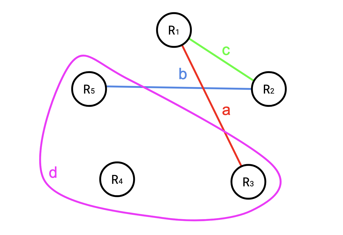
For example, say we had the following set of hyperedges for \(R = (R_1, R_2, R_3, R_4, R_5)\): \[ \begin{aligned} a &= \{R_1, R_3\} \cr b &= \{R_2, R_5\} \cr c &= \{R_1, R_2\} \cr d &= \{R_4, R_3, R_5\} \cr \end{aligned} \]
You might think of this like a table:
| \(e\) | \(R_1\) | \(R_2\) | \(R_3\) | \(R_4\) | \(R_5\) |
|---|---|---|---|---|---|
| \(a\) | X | X | |||
| \(b\) | X | X | |||
| \(c\) | X | X | |||
| \(d\) | X | X | X |
or a picture:
If \(w\) is such a covering, then Shearer’s Inequality states
\[ H[R] \le \sum_{e \in \mathcal{E}} w_e H[e] \]
where \(H[e]\) is the entropy of the random variables present in \(e\). Basically this says that if we’ve covered every constituent random variable, then taking the sum of all edges weighted by their assigned weights gives us an upper bound to the entropy in the original random variable.
Proof of Shearer’s Lemma
By the chain rule, for each \(e = \{q_1, \ldots, q_m\} \in \mathcal E\) (where each \(q_i\) is an index of an \(R_j\), and the \(q_i\)s themselves are increasing. \[ H[e] = \sum_{i=1}^m H[R_{q_i} | R_{q_{<i}}] \ge \sum_{i=1}^m H[R_{q_i} | R_{<q_i}] \]
The inequality holds because we are conditioning on more things in each term, which cannot increase the entropy.
Coming back to what we are trying to prove,
\[ H[R] \le \sum_{e \in \mathcal{E}} w_e H[e] \]
If we were to expand the LHS according to our other inequality, we would find that each \(H[R_i | R_{<i}]\) occurs exactly once. If we were to expand the RHS, since \(w\) is a cover, each \(H[R_i | R_{<i}]\) would occur with coefficient _at least_ 1, which prove Shearer.
Putting it all Together
For a relation \(X\), let \(R_X\) be a random variable representing selecting a row from \(X\) uniformly at random. Then
\[ H[R_X] = \sum_{x \in X} p(x) \log \frac1{p(x)} = \log |R_X| \]
Now take the join \(Q = X_1 \bowtie \ldots \bowtie X_n\). Projecting to the subset of the columns in \(Q\) which are in \(X_i\) gives a row from \(X_i\), due to the way the join works. So this is a new random variable which gives a row from \(R_i\). This one might not be uniform, but recall that entropy is maximized when we do have a uniform distribution, so we still have an upper bound.
Thus, we can partition up \(R_Q\) into a set of random variables like we did with Shearer, into the join tables: \[ R_Q = (R_{X_1}, \ldots, R_{X_n}) \] Like before, the right hand side contains all the information in the left hand side: since every column is present we can determine what the original row in \(Q\) was.
So, take a fractional edge cover \(w\) of the query graph, then, by Shearer: \[ \begin{aligned} H(R_Q) &= H(R_{X_1}, \ldots, R_{X_n}) \cr &\le \sum_{i=1}^n w_i H(R_{X_i}) \cr &\le \sum_{i=1}^n w_i \log |R_i| \cr &= \sum_{i=1}^n \log |R_i|^{w_i} \cr &= \log \prod_{i=1}^n |R_i|^{w_i} \cr \end{aligned} \]
so
\[ \begin{aligned} H(R_Q) &\le \log \prod_{i=1}^n |R_{X_i}|^{w_i} \cr \log|R_Q| &\le \log \prod_{i=1}^n |R_{X_i}|^{w_i} \cr |R_Q| &\le \prod_{i=1}^n |R_{X_i}|^{w_i} \cr \end{aligned} \] which is exactly the AGM bound.
Appendix: A Worst-Case Optimal Triangle Finder
A fully generic implementation of WCOJs has a lot of tedious bookkeeping, so we’ll just talk about a very simple triangle counter that doesn’t generalize (but could, with some elbow grease).
The simplest algorithm I’ve seen is “Algorithm 2” from Skew Strikes Back. It’s more or less the same as the presentation as in Leapfrog Triejoin.
To compute the query \[ Q(a, b, c) \leftarrow R(a, b), S(b, c), T(a, c). \] We’re going to first iterate over the values of \(a\) which are present in both \(R\) and \(T\), then for those values of \(a\) we will iterate over the values of \(b\) which are present in both \(R\) and \(S\) given that value of \(a\), and then finally iterate over the values of \(c\) which are present in \(S\) and \(T\) for those values of \(a\) and \(b\).
The algorithm is approximately this:
for each a in intersect(R, T):
  for each b in intersect(R[a], S):
    for each c in intersect(S[b], T[a]):
      emit((a, b, c))
The thing we’re doing here that’s different from a binary join approach is that we’re proceeding not by a relation at a time, but a variable at a time. We first fix \(a\), then \(b\), then \(c\), and then once there’s nothing left to fix, we must have found a triangle.
We could fix them in a different orders, which might have an impact on the runtime, but it turns out regardless of the ordering, this algorithm is worst-case optimal (and I point you at either of the two linked papers if you want more proof of that fact).
You can see an implementation here.
On my laptop this implementation ran about three times as fast as Postgres for a 2000 vertex random graph (and the gap only widens from there).
References
- Leapfrog Triejoin https://arxiv.org/abs/1210.0481
- Skew Strikes Back https://arxiv.org/abs/1310.3314